28 Math Attitudes with STEM Career Attainment (Dang, M., & Nylund-Gibson, K., 2017)
-
BY = Base Year (2002) - 10th grade
- Completed the baseline survey of high school sophomores in spring term 2002.
-
F1 = First follow up (2004) - 12th grade
- Most sample members were seniors, but some were dropouts or in other grades (early graduates or retained in an earlier grade).
F2 = Second follow up (2006) - Post-high-school follow-up
F3 = Third follow up (2012) - Kids are ~26yo
28.1 Item Descriptions
28.1.1 Base Year Covariates
English Proficiency BYS70A: How well student understands English (1 = Very well, 4 = Not at all) BYS70B: How well student speaks English (1 = Very well, 4 = Not at all) BYS70C: How well student reads English (1 = Very well, 4 = Not at all) BYS70D: How well 10th-grader writes English (1 = Very well, 4 = Not at all) BYTM12B: Student behind on schoolwork due to limited proficiency in English BYSTLANG: English if student’s native language
Demographics BYSEX: 1 = Male, 2 = Female BYRACE_R: All -5 since restricted BYSES2QU: SES Quartile
28.1.2 Base Year Indicators
BYS87A: When I do mathematics, I sometimes get totally absorbed BYS87C: Because doing mathematics is fun, I wouldn’t want to give it up BYS87F: Mathematics is important to me personally
BYS89A: I’m confident that I can do an excellent job on my math tests BYS89B: I’m certain I can understand the most difficult material presented in math texts BYS89L: I’m confident I can understand the most complex material presented by my math teacher BYS89R: I’m confident I can do an excellent job on my math assignments BYS89U: I’m certain I can master the skills being taught in my math class
Math Attitude BYS87 Items
Description: How much do you agree or disagree with the following statements?
Response options:
1 - Strongly agree
2 - Agree
3 - Disagree
4- Strongly disagree
Math Self-Efficacy BYS89/F1S18 Items
Description: How much do you agree or disagree with the following statements?
Response options:
1 - Almost never
2 - Sometimes
3 - Often
4- Almost always
28.1.3 F1 Indicators
F1S18A: I’m confident that I can do an excellent job on my math tests F1S18B: I’m certain I can understand the most difficult material presented in my math textbooks F1S18C: I’m confident I can understand the most complex material presented by my math teacher F1S18D: I’m confident I can do an excellent job on my math assignments F1S18E: I’m certain I can master the skills being taught in my math class
28.2 Read in data
Read in ELS .sav file:
View codebook:
#view_df(els_sav)Save subset:
els_subset <- els_sav %>%
  clean_names() %>%
  dplyr::select(
    stu_id, strat_id, psu,
    bys87a,bys87c,bys87f,bys89a,bys89b,bys89l,bys89r,bys89u,
    f1s18a,f1s18b,f1s18c,f1s18d,f1s18e,
    bys70a,bys70b,bys70c,bys70d,bystlang,bytm12b,bysex,byrace_r,
    byses2qu,f3onet2curr,f3onet6curr, f3bystemoc30, f3bytscwt
         ) %>%
  mutate(school = paste0(strat_id,psu))

view_df(els_subset)

#write_csv(els_subset, here("29-dang-lca-example", "els_data", "els_dang_analysis.csv"))
Read in ELS data file, els_dang_analysis.csv.
bys87_items <- c("bys87a","bys87c","bys87f")

f1s18_items <- c("f1s18a","f1s18b","f1s18c","f1s18d","f1s18e")

bys89_items <- c("bys89a","bys89b","bys89l","bys89r","bys89u")

els_data <- read_csv(
  here("29-dang-lca-example", "els_data", "els_dang_analysis.csv"),
  na = c("-9", "-8", "-6", "-5", "-4", "-7", "-1", "-3", "-2", "-99")
) %>%
  # Dichotomize English proficiency
  mutate(across(
    c(bys70a, bys70b, bys70c, bys70d),
    ~ case_when(. %in% c(1, 2) ~ 1,
                . %in% c(3, 4) ~ 0,
                TRUE ~ NA_real_)
  )) %>%
  mutate(across(
    c(f3onet2curr),
    ~ case_when(is.na(.) ~ NA_real_,
                . %in% c(11, 15, 17, 19, 25, 45, 51) ~ 1,
                TRUE ~ 0)
  )) %>%
  mutate(female = case_match(bysex,
                             2 ~ 1,
                             1 ~ 0,
                             .default = NA_real_)) %>%
  mutate(ses_dichotomized = case_match(
    byses2qu,
    1 ~ 1,
    NA ~ NA,
    .default = 0
  )) %>%
  mutate(across(
    all_of(bys87_items),
    ~ case_when(. %in% c(1, 2) ~ 1,
                . %in% c(3, 4) ~ 0,
                TRUE ~ NA_real_)
  )) %>%
  mutate(across(all_of(c(
    bys89_items, f1s18_items
  )), ~ case_when(
    . %in% c(1, 2) ~ 0,
    . %in% c(3, 4) ~ 1,
    TRUE ~ NA_real_
  )))

summary(els_data)
#>      stu_id          strat_id          psu
#>  Min.   :101101   Min.   :101.0   Min.   :1.000
#>  1st Qu.:190106   1st Qu.:190.0   1st Qu.:1.000
#>  Median :281116   Median :281.0   Median :2.000
#>  Mean   :279543   Mean   :279.4   Mean   :1.557
#>  3rd Qu.:369205   3rd Qu.:369.0   3rd Qu.:2.000
#>  Max.   :461234   Max.   :461.0   Max.   :3.000
#>
#>      bys87a           bys87c           bys87f
#>  Min.   :0.0000   Min.   :0.0000   Min.   :0.0000
#>  1st Qu.:0.0000   1st Qu.:0.0000   1st Qu.:0.0000
#>  Median :1.0000   Median :0.0000   Median :1.0000
#>  Mean   :0.5181   Mean   :0.3387   Mean   :0.5108
#>  3rd Qu.:1.0000   3rd Qu.:1.0000   3rd Qu.:1.0000
#>  Max.   :1.0000   Max.   :1.0000   Max.   :1.0000
#>  NAs    :4457     NAs    :4523     NAs    :4439
#>      bys89a           bys89b           bys89l
#>  Min.   :0.0000   Min.   :0.0000   Min.   :0.0000
#>  1st Qu.:0.0000   1st Qu.:0.0000   1st Qu.:0.0000
#>  Median :0.0000   Median :0.0000   Median :0.0000
#>  Mean   :0.4436   Mean   :0.3987   Mean   :0.4482
#>  3rd Qu.:1.0000   3rd Qu.:1.0000   3rd Qu.:1.0000
#>  Max.   :1.0000   Max.   :1.0000   Max.   :1.0000
#>  NAs    :4806     NAs    :4765     NAs    :5150
#>      bys89r           bys89u          f1s18a
#>  Min.   :0.0000   Min.   :0.000   Min.   :0.0000
#>  1st Qu.:0.0000   1st Qu.:0.000   1st Qu.:0.0000
#>  Median :1.0000   Median :1.000   Median :0.0000
#>  Mean   :0.5168   Mean   :0.534   Mean   :0.4841
#>  3rd Qu.:1.0000   3rd Qu.:1.000   3rd Qu.:1.0000
#>  Max.   :1.0000   Max.   :1.000   Max.   :1.0000
#>  NAs    :5374     NAs    :5536    NAs    :5860
#>      f1s18b           f1s18c           f1s18d
#>  Min.   :0.0000   Min.   :0.0000   Min.   :0.0000
#>  1st Qu.:0.0000   1st Qu.:0.0000   1st Qu.:0.0000
#>  Median :0.0000   Median :0.0000   Median :1.0000
#>  Mean   :0.4093   Mean   :0.4506   Mean   :0.6541
#>  3rd Qu.:1.0000   3rd Qu.:1.0000   3rd Qu.:1.0000
#>  Max.   :1.0000   Max.   :1.0000   Max.   :1.0000
#>  NAs    :5883     NAs    :5907     NAs    :5913
#>      f1s18e           bys70a           bys70b
#>  Min.   :0.0000   Min.   :0.0000   Min.   :0.0000
#>  1st Qu.:0.0000   1st Qu.:1.0000   1st Qu.:1.0000
#>  Median :1.0000   Median :1.0000   Median :1.0000
#>  Mean   :0.5899   Mean   :0.9522   Mean   :0.9272
#>  3rd Qu.:1.0000   3rd Qu.:1.0000   3rd Qu.:1.0000
#>  Max.   :1.0000   Max.   :1.0000   Max.   :1.0000
#>  NAs    :5903     NAs    :13916    NAs    :13904
#>      bys70c           bys70d          bystlang
#>  Min.   :0.0000   Min.   :0.0000   Min.   :0.0000
#>  1st Qu.:1.0000   1st Qu.:1.0000   1st Qu.:1.0000
#>  Median :1.0000   Median :1.0000   Median :1.0000
#>  Mean   :0.9222   Mean   :0.8954   Mean   :0.8304
#>  3rd Qu.:1.0000   3rd Qu.:1.0000   3rd Qu.:1.0000
#>  Max.   :1.0000   Max.   :1.0000   Max.   :1.0000
#>  NAs    :13923    NAs    :13913    NAs    :953
#>     bytm12b            bysex       byrace_r
#>  Min.   :0.00000   Min.   :1.000   Mode:logical
#>  1st Qu.:0.00000   1st Qu.:1.000   NAs :16197
#>  Median :0.00000   Median :2.000
#>  Mean   :0.03861   Mean   :1.502
#>  3rd Qu.:0.00000   3rd Qu.:2.000
#>  Max.   :1.00000   Max.   :2.000
#>  NAs    :11924     NAs    :827
#>     byses2qu      f3onet2curr    f3onet6curr
#>  Min.   :1.000   Min.   :0.000   Mode:logical
#>  1st Qu.:2.000   1st Qu.:0.000   NAs :16197
#>  Median :3.000   Median :0.000
#>  Mean   :2.574   Mean   :0.271
#>  3rd Qu.:4.000   3rd Qu.:1.000
#>  Max.   :4.000   Max.   :1.000
#>  NAs    :953     NAs    :3401
#>    f3bytscwt          school         female
#>  Min.   :   0.0   Min.   :1011   Min.   :0.0000
#>  1st Qu.:   0.0   1st Qu.:1901   1st Qu.:0.0000
#>  Median : 150.7   Median :2811   Median :1.0000
#>  Mean   : 200.6   Mean   :2795   Mean   :0.5021
#>  3rd Qu.: 310.3   3rd Qu.:3692   3rd Qu.:1.0000
#>  Max.   :2163.2   Max.   :4612   Max.   :1.0000
#>                                  NAs    :827
#>  ses_dichotomized
#>  Min.   :0.0000
#>  1st Qu.:0.0000
#>  Median :0.0000
#>  Mean   :0.2362
#>  3rd Qu.:0.0000
#>  Max.   :1.0000
#>  NAs    :953

summary(factor(els_data$bys70a))
#>     0     1   NAs
#>   109  2172 13916
summary(factor(els_data$bys70b))
#>     0     1   NAs
#>   167  2126 13904
summary(factor(els_data$bys70c))
#>     0     1   NAs
#>   177  2097 13923
summary(factor(els_data$bys70d))
#>     0     1   NAs
#>   239  2045 13913
summary(factor(els_data$bystlang))
#>     0     1   NAs
#>  2586 12658   953
summary(factor(els_data$f3onet2curr))
#>    0    1  NAs
#> 9328 3468 3401
summary(factor(els_data$female))
#>    0    1  NAs
#> 7653 7717  827
summary(factor(els_data$bysex))
#>    1    2  NAs
#> 7653 7717  827
summary(factor(els_data$byses2qu))
#>    1    2    3    4  NAs
#> 3600 3590 3753 4301  953
summary(factor(els_data$ses_dichotomized))
#>     0     1   NAs
#> 11644  3600   953
28.3 Descriptive Statistics
Linguistic Minority
“Respondents were classified as linguistic minority if they reported that English was not their first language and they responded that they read,speak, write, and/or understand English well. Respondents were classified as native English speakers if they indicated they speak English as a first language and they read, speak, write, and understand English well. Using these criteria, among the total 8,790 students, 7,490 (85.2%) were classified as native English speakers, 1,040 (11.8%) were classified as linguistic minority students, and 260 (3.0%) were classified as ELLs.” (page 8)
BYS70A: How well student understands English (1 = Very well, 4 = Not at all) but already dichotomized BYS70B: How well student speaks English (1 = Very well, 4 = Not at all) but already dichotomized BYS70C: How well student reads English (1 = Very well, 4 = Not at all) but already dichotomized BYS70D: How well 10th-grader writes English (1 = Very well, 4 = Not at all) but already dichotomized BYTM12B: Student behind on schoolwork due to limited proficiency in English
ling_min <- els_subset %>%
  mutate(across(where(is.labelled), zap_labels)) %>%
  replace_with_na_all(condition = ~.x %in% c(-9,-8,-6,-5,-4,-7,-1,-3,-2,-99)) %>%
  select(bys70a,bys70b,bys70c,bys70d,bytm12b)

f <- All(ling_min) ~ Mean + SD + Min + Median + Max + Histogram

datasummary(f, els_subset, output="markdown")

summary(factor(ling_min$bys70a))
summary(factor(ling_min$bys70b))
summary(factor(ling_min$bys70c))
summary(factor(ling_min$bys70d))
summary(factor(ling_min$bytm12b))


# Trying to create the linguistic minority variable:
ling_minority_var <- els_data %>%
  mutate(
    lang_status = case_when(
      # Condition A: Native English Speaker
      # Native language is English AND proficient in all 4 domains
      bystlang == 1 & bys70a == 1 & bys70b == 1 & bys70c == 1 & bys70d == 1
        ~ "Native English Speaker",

      # Condition B: Linguistic Minority
      # Not native English speaker, BUT reads, speaks, writes, and/or understands well
      bystlang == 0 & (bys70a == 1 | bys70b == 1 | bys70c == 1 | bys70d == 1)
        ~ "Linguistic Minority",

      # Condition C: ELL (English Language Learner)
      # Not native English speaker AND has limited proficiency / behind in schoolwork
      bystlang == 0 & (bytm12b == 1 | (bys70a != 1 & bys70b != 1 & bys70c != 1 & bys70d != 1))
        ~ "ELL",

      # If data is missing for vital logic pieces, preserve it as NA
      TRUE ~ NA_character_
    ),
    # Convert to a factor for clean modeling/summaries later
    lang_status = factor(lang_status, levels = c("Native English Speaker", "Linguistic Minority", "ELL"))
  )


summary(factor(ling_minority_var$lang_status))
math_subset <- els_data %>%
  select(bys87a,bys87c,bys87f,bys89a,bys89b,bys89l,bys89r,bys89u,f1s18a,f1s18b,f1s18c,f1s18d,f1s18e)
Descriptive
f <- All(math_subset) ~ Mean + SD + Min + Median + Max + Histogram

datasummary(f, els_data, output="markdown")| Mean | SD | Min | Median | Max | Histogram | |
|---|---|---|---|---|---|---|
| bys87a | 0.52 | 0.50 | 0.00 | 1.00 | 1.00 | ▇▇ |
| bys87c | 0.34 | 0.47 | 0.00 | 0.00 | 1.00 | ▇▄ |
| bys87f | 0.51 | 0.50 | 0.00 | 1.00 | 1.00 | ▇▇ |
| bys89a | 0.44 | 0.50 | 0.00 | 0.00 | 1.00 | ▇▆ |
| bys89b | 0.40 | 0.49 | 0.00 | 0.00 | 1.00 | ▇▅ |
| bys89l | 0.45 | 0.50 | 0.00 | 0.00 | 1.00 | ▇▆ |
| bys89r | 0.52 | 0.50 | 0.00 | 1.00 | 1.00 | ▇▇ |
| bys89u | 0.53 | 0.50 | 0.00 | 1.00 | 1.00 | ▆▇ |
| f1s18a | 0.48 | 0.50 | 0.00 | 0.00 | 1.00 | ▇▇ |
| f1s18b | 0.41 | 0.49 | 0.00 | 0.00 | 1.00 | ▇▅ |
| f1s18c | 0.45 | 0.50 | 0.00 | 0.00 | 1.00 | ▇▆ |
| f1s18d | 0.65 | 0.48 | 0.00 | 1.00 | 1.00 | ▄▇ |
| f1s18e | 0.59 | 0.49 | 0.00 | 1.00 | 1.00 | ▅▇ |
Weighted average
bys87_items <- c("bys87a","bys87c","bys87f")

f1s18_items <- c("f1s18a","f1s18b","f1s18c","f1s18d","f1s18e")

bys89_items <- c("bys89a","bys89b","bys89l","bys89r","bys89u")

math_binary_weighted <- els_data %>%
  summarise(across(c(all_of(bys87_items), all_of(c(bys89_items, f1s18_items))),
                   list(
                     w_mean = ~ weighted.mean(.x, f3bytscwt, na.rm = TRUE),
                     w_sd = ~ {
                       keep <- !is.na(.x) & !is.na(f3bytscwt)
                       x <- .x[keep]
                       w_raw <- f3bytscwt[keep]
                       w <- w_raw / sum(w_raw)
                       mu <- sum(w * x)
                       sqrt(sum(w * (x - mu)^2))
                     }
                   ),
                   .names = "{.col}_{.fn}"
  )) %>%
  pivot_longer(
    cols = everything(),
    names_to = c("item", ".value"),
    names_pattern = "(.*)_(w_mean|w_sd)"
  )

math_binary_weighted
#> # A tibble: 13 × 3
#>    item   w_mean  w_sd
#>    <chr>   <dbl> <dbl>
#>  1 bys87a  0.508 0.500
#>  2 bys87c  0.333 0.471
#>  3 bys87f  0.504 0.500
#>  4 bys89a  0.450 0.497
#>  5 bys89b  0.401 0.490
#>  6 bys89l  0.452 0.498
#>  7 bys89r  0.520 0.500
#>  8 bys89u  0.538 0.499
#>  9 f1s18a  0.483 0.500
#> 10 f1s18b  0.407 0.491
#> 11 f1s18c  0.452 0.498
#> 12 f1s18d  0.655 0.475
#> 13 f1s18e  0.589 0.492
library(tidyverse)
library(gt)

item_labels <- tibble(
  item = c(
    "bys87a", "bys87c", "bys87f",
    "f1s18a", "f1s18b", "f1s18c", "f1s18d", "f1s18e",
    "bys89a", "bys89b", "bys89l", "bys89r", "bys89u"
  ),
  scale = c(
    rep("Math attitudes", 3),
    rep("Math self-efficacy", 5),
    rep("Math experiences", 5)
  ),
  item_label = c(
    "I enjoy math",
    "Math is one of my best subjects",
    "Math is useful for my future",
    "Certain I can understand math",
    "Certain I can do well in math",
    "Certain I can learn math",
    "Certain I can master math skills",
    "Certain I can complete math assignments",
    "Took advanced math",
    "Participated in math club",
    "Worked hard in math",
    "Talked with teacher about math",
    "Planned to take more math"
  )
)

math_binary_weighted_table <- math_binary_weighted %>%
  left_join(item_labels, by = "item") %>%
  mutate(
    percent_endorsed = w_mean * 100,
    sd = w_sd
  ) %>%
  select(scale, item, item_label, percent_endorsed, sd)

math_binary_weighted_table %>%
  gt(groupname_col = "scale") %>%
  cols_label(
    item = "Item",
    item_label = "Item wording",
    percent_endorsed = "% endorsed",
    sd = "SD"
  ) %>%
  fmt_number(
    columns = c(percent_endorsed, sd),
    decimals = 2
  ) %>%
  tab_header(
    title = "Weighted Descriptive Statistics for Binary Math Indicators",
    subtitle = "Weighted means represent the percentage endorsing the focal response category"
  ) %>%
  tab_options(
    table.font.size = 13,
    heading.title.font.size = 16,
    heading.subtitle.font.size = 12,
    row_group.font.weight = "bold",
    column_labels.font.weight = "bold"
)| Weighted Descriptive Statistics for Binary Math Indicators | |||
| Weighted means represent the percentage endorsing the focal response category | |||
| Item | Item wording | % endorsed | SD |
|---|---|---|---|
| Math attitudes | |||
| bys87a | I enjoy math | 50.79 | 0.50 |
| bys87c | Math is one of my best subjects | 33.27 | 0.47 |
| bys87f | Math is useful for my future | 50.39 | 0.50 |
| Math experiences | |||
| bys89a | Took advanced math | 44.97 | 0.50 |
| bys89b | Participated in math club | 40.10 | 0.49 |
| bys89l | Worked hard in math | 45.20 | 0.50 |
| bys89r | Talked with teacher about math | 51.97 | 0.50 |
| bys89u | Planned to take more math | 53.76 | 0.50 |
| Math self-efficacy | |||
| f1s18a | Certain I can understand math | 48.28 | 0.50 |
| f1s18b | Certain I can do well in math | 40.74 | 0.49 |
| f1s18c | Certain I can learn math | 45.17 | 0.50 |
| f1s18d | Certain I can master math skills | 65.52 | 0.48 |
| f1s18e | Certain I can complete math assignments | 58.94 | 0.49 |
Proportions
# Dichotomize
math_binary <- els_data %>%
  select(bys87_items,bys89_items,f1s18_items, f3bytscwt, f3onet2curr, bystlang, stu_id)

# Set up data to find proportions of binary indicators
ds <- math_binary %>%
  select(-f3bytscwt, -bystlang, -stu_id, -f3onet2curr) %>%
  pivot_longer(
    cols = everything(),
    names_to = "variable",
    values_to = "value"
  )

# Create table of variables and counts, then find proportions and round to 3 decimal places
prop_df <- ds %>%
  count(variable, value) %>%
  group_by(variable) %>%
  mutate(prop = n / sum(n)) %>%
  ungroup() %>%
  mutate(prop = round(prop, 3))


# Make it a gt() table
prop_table <- prop_df %>%
  gt(groupname_col = "variable", rowname_col = "value") %>%
  tab_stubhead(label = md("*Values*")) %>%
  tab_header(
    md(
      "Variable Proportions"
    )
  ) %>%
  cols_label(
    variable = md("*Variable*"),
    value = md("*Value*"),
    n = md("*N*"),
    prop = md("*Proportion*")
  )

prop_table| Variable Proportions | ||
| Values | N | Proportion |
|---|---|---|
| bys87a | ||
| 0 | 5658 | 0.349 |
| 1 | 6082 | 0.376 |
| NA | 4457 | 0.275 |
| bys87c | ||
| 0 | 7720 | 0.477 |
| 1 | 3954 | 0.244 |
| NA | 4523 | 0.279 |
| bys87f | ||
| 0 | 5752 | 0.355 |
| 1 | 6006 | 0.371 |
| NA | 4439 | 0.274 |
| bys89a | ||
| 0 | 6338 | 0.391 |
| 1 | 5053 | 0.312 |
| NA | 4806 | 0.297 |
| bys89b | ||
| 0 | 6874 | 0.424 |
| 1 | 4558 | 0.281 |
| NA | 4765 | 0.294 |
| bys89l | ||
| 0 | 6096 | 0.376 |
| 1 | 4951 | 0.306 |
| NA | 5150 | 0.318 |
| bys89r | ||
| 0 | 5230 | 0.323 |
| 1 | 5593 | 0.345 |
| NA | 5374 | 0.332 |
| bys89u | ||
| 0 | 4968 | 0.307 |
| 1 | 5693 | 0.351 |
| NA | 5536 | 0.342 |
| f1s18a | ||
| 0 | 5333 | 0.329 |
| 1 | 5004 | 0.309 |
| NA | 5860 | 0.362 |
| f1s18b | ||
| 0 | 6092 | 0.376 |
| 1 | 4222 | 0.261 |
| NA | 5883 | 0.363 |
| f1s18c | ||
| 0 | 5653 | 0.349 |
| 1 | 4637 | 0.286 |
| NA | 5907 | 0.365 |
| f1s18d | ||
| 0 | 3557 | 0.220 |
| 1 | 6727 | 0.415 |
| NA | 5913 | 0.365 |
| f1s18e | ||
| 0 | 4222 | 0.261 |
| 1 | 6072 | 0.375 |
| NA | 5903 | 0.364 |
psych::describe(math_binary)
#>             vars     n      mean        sd    median
#> bys87a         1 11740      0.52      0.50      1.00
#> bys87c         2 11674      0.34      0.47      0.00
#> bys87f         3 11758      0.51      0.50      1.00
#> bys89a         4 11391      0.44      0.50      0.00
#> bys89b         5 11432      0.40      0.49      0.00
#> bys89l         6 11047      0.45      0.50      0.00
#> bys89r         7 10823      0.52      0.50      1.00
#> bys89u         8 10661      0.53      0.50      1.00
#> f1s18a         9 10337      0.48      0.50      0.00
#> f1s18b        10 10314      0.41      0.49      0.00
#> f1s18c        11 10290      0.45      0.50      0.00
#> f1s18d        12 10284      0.65      0.48      1.00
#> f1s18e        13 10294      0.59      0.49      1.00
#> f3bytscwt     14 16197    200.58    212.77    150.69
#> f3onet2curr   15 12796      0.27      0.44      0.00
#> bystlang      16 15244      0.83      0.38      1.00
#> stu_id        17 16197 279542.70 104263.77 281116.00
#>               trimmed       mad    min       max     range
#> bys87a           0.52      0.00      0      1.00      1.00
#> bys87c           0.30      0.00      0      1.00      1.00
#> bys87f           0.51      0.00      0      1.00      1.00
#> bys89a           0.43      0.00      0      1.00      1.00
#> bys89b           0.37      0.00      0      1.00      1.00
#> bys89l           0.44      0.00      0      1.00      1.00
#> bys89r           0.52      0.00      0      1.00      1.00
#> bys89u           0.54      0.00      0      1.00      1.00
#> f1s18a           0.48      0.00      0      1.00      1.00
#> f1s18b           0.39      0.00      0      1.00      1.00
#> f1s18c           0.44      0.00      0      1.00      1.00
#> f1s18d           0.69      0.00      0      1.00      1.00
#> f1s18e           0.61      0.00      0      1.00      1.00
#> f3bytscwt      167.57    223.42      0   2163.17   2163.17
#> f3onet2curr      0.21      0.00      0      1.00      1.00
#> bystlang         0.91      0.00      0      1.00      1.00
#> stu_id      279551.71 133070.76 101101 461234.00 360133.00
#>              skew kurtosis     se
#> bys87a      -0.07    -1.99   0.00
#> bys87c       0.68    -1.54   0.00
#> bys87f      -0.04    -2.00   0.00
#> bys89a       0.23    -1.95   0.00
#> bys89b       0.41    -1.83   0.00
#> bys89l       0.21    -1.96   0.00
#> bys89r      -0.07    -2.00   0.00
#> bys89u      -0.14    -1.98   0.00
#> f1s18a       0.06    -2.00   0.00
#> f1s18b       0.37    -1.86   0.00
#> f1s18c       0.20    -1.96   0.00
#> f1s18d      -0.65    -1.58   0.00
#> f1s18e      -0.37    -1.87   0.00
#> f3bytscwt    1.43     3.18   1.67
#> f3onet2curr  1.03    -0.94   0.00
#> bystlang    -1.76     1.10   0.00
#> stu_id       0.00    -1.20 819.25
# Item labels
item_labels <- tibble(
  variable = c(
    "bys87a", "bys87c", "bys87f",
    "bys89a", "bys89b", "bys89l", "bys89r", "bys89u",
    "f1s18a", "f1s18b", "f1s18c", "f1s18d", "f1s18e"
  ),
  scale = c(
    rep("Math attitudes", 3),
    rep("Math experiences", 5),
    rep("Math self-efficacy", 5)
  ),
  item_label = c(
    "I enjoy math",
    "Math is one of my best subjects",
    "Math is useful for my future",
    "Took advanced math",
    "Participated in math club",
    "Worked hard in math",
    "Talked with teacher about math",
    "Planned to take more math",
    "Certain I can understand math",
    "Certain I can do well in math",
    "Certain I can learn math",
    "Certain I can master math skills",
    "Certain I can complete math assignments"
  )
)

prop_table_data <- math_binary %>%
  select(all_of(c(bys87_items, bys89_items, f1s18_items))) %>%
  pivot_longer(
    cols = everything(),
    names_to = "variable",
    values_to = "value"
  ) %>%
  filter(!is.na(value)) %>%
  count(variable, value, name = "n") %>%
  group_by(variable) %>%
  mutate(
    total_n = sum(n),
    prop = n / total_n
  ) %>%
  ungroup() %>%
  left_join(item_labels, by = "variable") %>%
  mutate(
    value_label = case_when(
      value == 1 ~ "1 = endorsed",
      value == 0 ~ "0 = not endorsed"
    )
  ) %>%
  select(scale, variable, item_label, value_label, n, total_n, prop)
prop_endorsed_table <- prop_table_data %>%
  filter(value_label == "1 = endorsed") %>%
  select(scale, variable, item_label, n, total_n, prop) %>%
  gt(groupname_col = "scale") %>%
  cols_label(
    variable = "Item",
    item_label = "Item wording",
    n = "Endorsed N",
    total_n = "Valid N",
    prop = "% endorsed"
  ) %>%
  fmt_percent(
    columns = prop,
    decimals = 1
  ) %>%
  tab_header(
    title = "Unweighted Endorsement Rates for Binary Math Indicators",
    subtitle = "Endorsement refers to the response category recoded as 1"
  ) %>%
  tab_options(
    table.font.size = 13,
    heading.title.font.size = 16,
    heading.subtitle.font.size = 12,
    row_group.font.weight = "bold",
    column_labels.font.weight = "bold"
  )

prop_endorsed_table| Unweighted Endorsement Rates for Binary Math Indicators | ||||
| Endorsement refers to the response category recoded as 1 | ||||
| Item | Item wording | Endorsed N | Valid N | % endorsed |
|---|---|---|---|---|
| Math attitudes | ||||
| bys87a | I enjoy math | 6082 | 11740 | 51.8% |
| bys87c | Math is one of my best subjects | 3954 | 11674 | 33.9% |
| bys87f | Math is useful for my future | 6006 | 11758 | 51.1% |
| Math experiences | ||||
| bys89a | Took advanced math | 5053 | 11391 | 44.4% |
| bys89b | Participated in math club | 4558 | 11432 | 39.9% |
| bys89l | Worked hard in math | 4951 | 11047 | 44.8% |
| bys89r | Talked with teacher about math | 5593 | 10823 | 51.7% |
| bys89u | Planned to take more math | 5693 | 10661 | 53.4% |
| Math self-efficacy | ||||
| f1s18a | Certain I can understand math | 5004 | 10337 | 48.4% |
| f1s18b | Certain I can do well in math | 4222 | 10314 | 40.9% |
| f1s18c | Certain I can learn math | 4637 | 10290 | 45.1% |
| f1s18d | Certain I can master math skills | 6727 | 10284 | 65.4% |
| f1s18e | Certain I can complete math assignments | 6072 | 10294 | 59.0% |
28.4 Math Attitudes & Self-Efficacy
28.4.1 Full Sample
Basic analysis
basic_t1  <- mplusObject(

   TITLE = glue("Basic - T1"),

   VARIABLE =
    "categorical = bys87a,bys87c,bys87f,bys89a,
    bys89b,bys89l,bys89r,bys89u;
     usevar = bys87a,bys87c,bys87f,bys89a,
    bys89b,bys89l,bys89r,bys89u;

    WEIGHT = f3bytscwt;",

  ANALYSIS =
   "type = basic;",

  OUTPUT = "sampstat;",

  usevariables = colnames(math_binary),
  rdata = math_binary)

basic_t1_fit <- mplusModeler(basic_t1,
                 dataout=here("basic.dat"),
                 modelout=here("basic.inp"),
                 check=TRUE, run = TRUE, hashfilename = FALSE)
Enumeration
if (!dir.exists("enumeration")) {
  dir.create("enumeration", recursive = TRUE)
}

t1_enum <- lapply(1:6, function(k) {
  enum_t1  <- mplusObject(

   TITLE = glue("Class {k} Math Attitudes & Efficacy - T1"),

   VARIABLE = glue(
    "categorical = bys87a,bys87c,bys87f,bys89a,
    bys89b,bys89l,bys89r,bys89u;
     usevar = bys87a,bys87c,bys87f,bys89a,
    bys89b,bys89l,bys89r,bys89u;

    WEIGHT = f3bytscwt;

     classes = c({k});"),

  ANALYSIS =
   "estimator = mlr;
    type = mixture;
    starts = 500 100;
    processors = 12;",

  OUTPUT = "sampstat residual tech11 tech14;",

  usevariables = colnames(math_binary),
  rdata = math_binary)

enum_t1_fit <- mplusModeler(enum_t1,
                 dataout=here("enumeration","enum.dat"),
                 modelout=glue(here("enumeration","c{k}_math_weighted.inp")),
                 check=TRUE, run = TRUE, hashfilename = FALSE)
})
Model Fit Summary
source(here("29-dang-lca-example","functions", "extract_mplus_info.R"))
source(here("29-dang-lca-example","functions","enum_table.R"))

# Define the directory where all of the .out files are located.
output_dir <- here("29-dang-lca-example","enumeration")

# Get all .out files
output_files <- list.files(output_dir, pattern = "\\.out$", full.names = TRUE)

# Process all .out files into one dataframe
final_data <- map_dfr(output_files, extract_mplus_info_extended)

# Extract Sample_Size from final_data
sample_size <- unique(final_data$Sample_Size)

output_enum <- readModels(here("29-dang-lca-example","enumeration"), quiet = TRUE)

enum_table_weights(output_enum)| Model Fit Summary Table1 | ||||||||||
| Classes | Par | LL | % Converged | % Replicated |
Model Fit Indices
|
LRTs
|
Smallest Class
|
|||
|---|---|---|---|---|---|---|---|---|---|---|
| BIC | aBIC | CAIC | AWE | VLMR | n (%) | |||||
| Class 1 Math Attitudes & Efficacy - T1 | 8 | −62,206.05 | 100% | 100% | 124,487.34 | 124,461.91 | 124,495.34 | 124,586.58 | – | 12146 (100%) |
| Class 2 Math Attitudes & Efficacy - T1 | 17 | −48,467.32 | 100% | 100% | 97,094.51 | 97,040.49 | 97,111.51 | 97,305.39 | <.001 | 5607 (46.2%) |
| Class 3 Math Attitudes & Efficacy - T1 | 26 | −47,104.20 | 55% | 62% | 94,452.93 | 94,370.30 | 94,478.93 | 94,775.45 | <.001 | 3782 (31.1%) |
| Class 4 Math Attitudes & Efficacy - T1 | 35 | −45,812.59 | 78% | 100% | 91,954.35 | 91,843.12 | 91,989.35 | 92,388.51 | <.001 | 2252 (18.5%) |
| Class 5 Math Attitudes & Efficacy - T1 | 44 | −45,344.55 | 76% | 92% | 91,102.92 | 90,963.09 | 91,146.92 | 91,648.73 | <.001 | 1584 (13%) |
| Class 6 Math Attitudes & Efficacy - T1 | 53 | −45,109.87 | 41% | 93% | 90,718.20 | 90,549.77 | 90,771.20 | 91,375.65 | 0.01 | 899 (7.4%) |
| 1 Note. Par = Parameters; LL = model log likelihood; BIC = Bayesian information criterion; aBIC = sample size adjusted BIC; CAIC = consistent Akaike information criterion; AWE = approximate weight of evidence criterion; VLMR = Vuong-Lo-Mendell-Rubin adjusted likelihood ratio test p-value; cmPk = approximate correct model probability. | ||||||||||
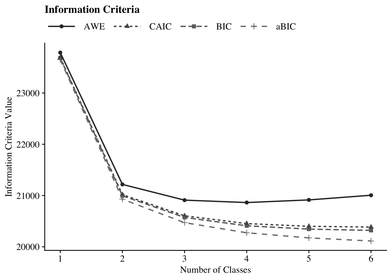
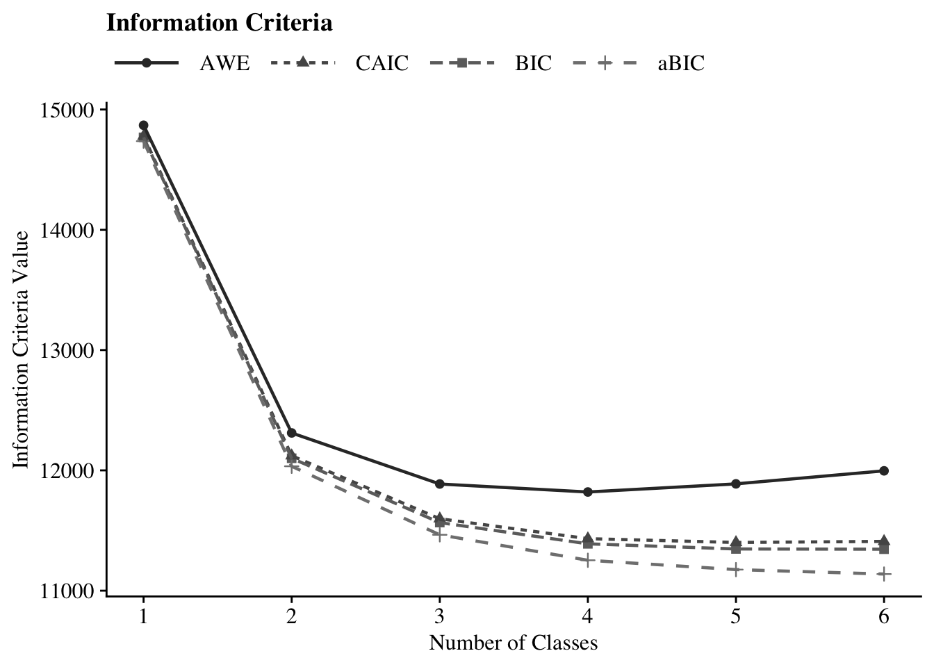
IC Plot
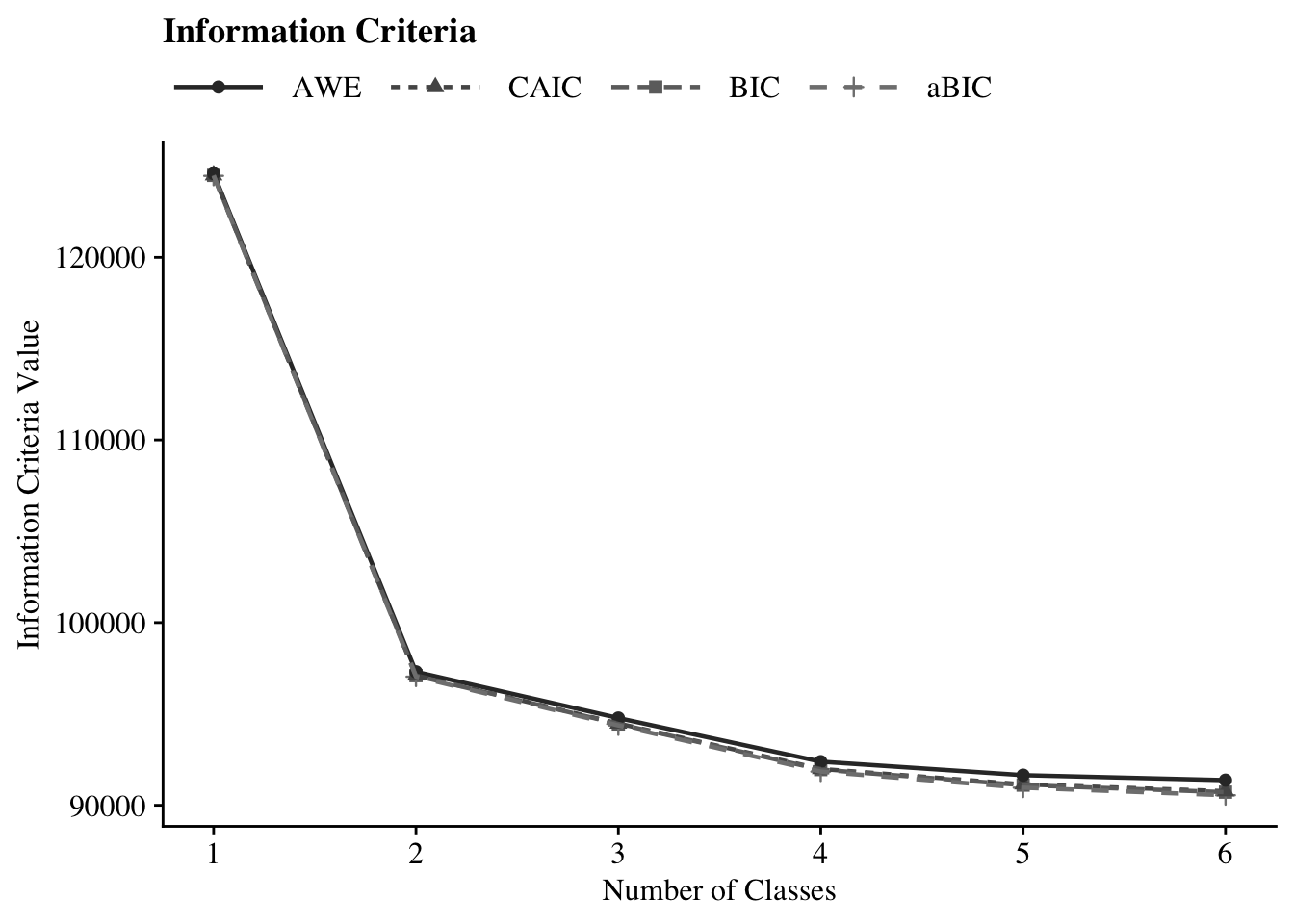
Plot LCA:
source(here("29-dang-lca-example", "functions","plot_lca.R"))

plot_lca(output_enum$c4_math_weighted.out)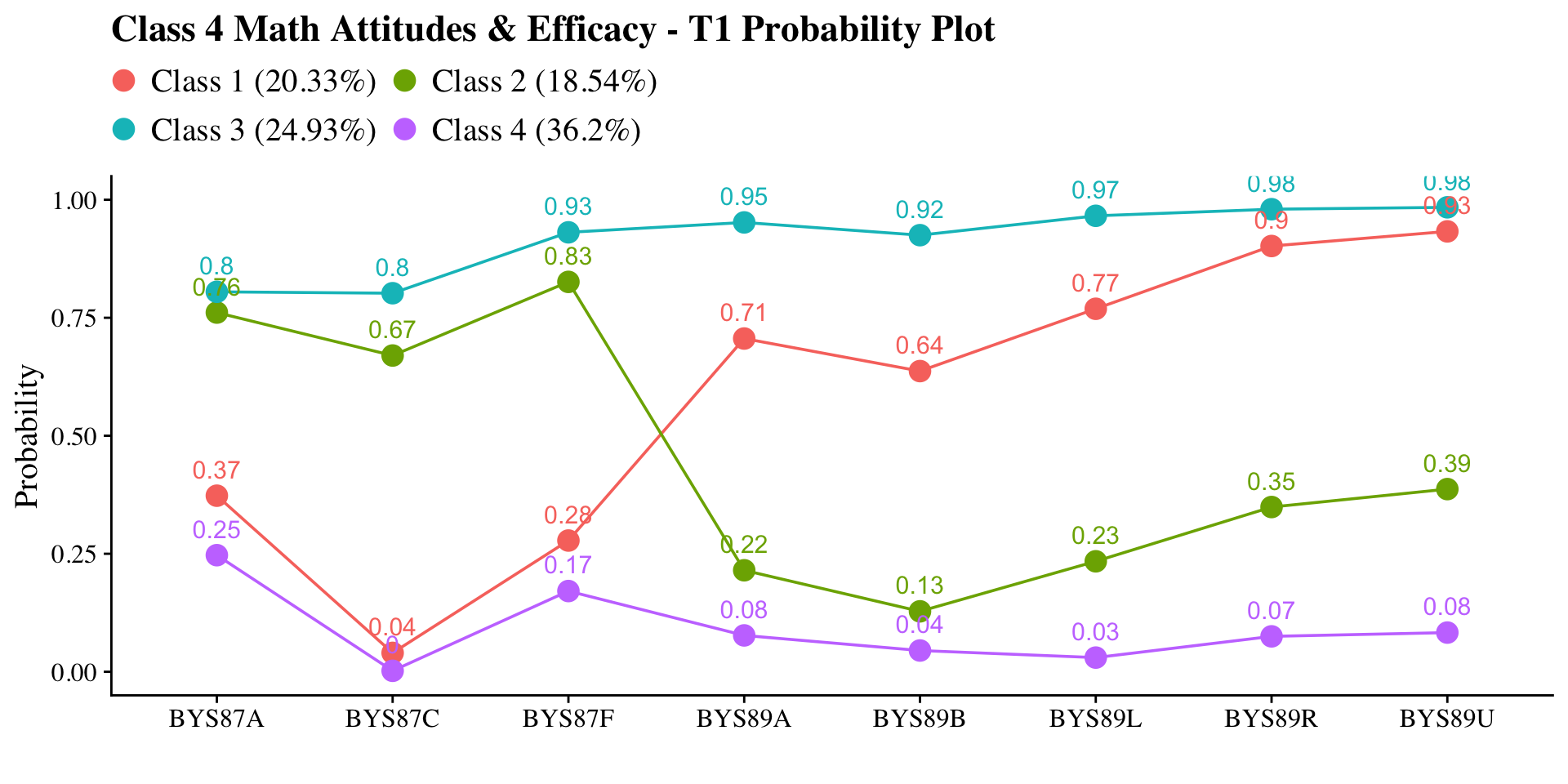
28.5 Manual ML Three-step
28.5.1 Step 1 - Class Enumeration w/ Auxiliary Specification
This step is done after class enumeration (or after you have selected the best latent class model). In this example, the four class model was the best. Now, we re-estimate the five-class model using optseed for efficiency. The difference here is the SAVEDATA command, where I can save the posterior probabilities and the modal class assignment that will be used in steps two and three.
step1  <- mplusObject(

  TITLE = "Step 1 - Three-Step",

  VARIABLE =
  "categorical = bys87a,bys87c,bys87f,bys89a,
    bys89b,bys89l,bys89r,bys89u;
   usevar = bys87a,bys87c,bys87f,bys89a,
    bys89b,bys89l,bys89r,bys89u;

   classes = c(4);

   auxiliary =
   female
   ses_dichotomized
   f3onet2curr;

  WEIGHT = f3bytscwt;",

  ANALYSIS =
   "estimator = mlr;
    type = mixture;
    starts = 0;
    optseed = 399671;",

  SAVEDATA =
   "File=savedata.dat;
    Save=cprob;",

  OUTPUT = "residual tech11 tech14",

  usevariables = colnames(els_data),
  rdata = els_data)

step1_fit <- mplusModeler(step1,
                            dataout=here("29-dang-lca-example", "three_step", "Step1.dat"),
                            modelout=here("29-dang-lca-example", "three_step", "one.inp") ,
                            check=TRUE, run = TRUE, hashfilename = FALSE)
Plot LCA
Class 1 = Low Math Attitudes, High Self-Efficacy (20.33%) Class 2 = High Math Attitudes, Low Self-Efficacy (18.546%) Class 3 = High Math Attitudes, High Self-Efficacy (24.93%) Class 4 = Low Math Attitudes, Low Self-Efficacy (36.2%)
source(here("29-dang-lca-example", "functions", "plot_lca.R"))
output_one <- readModels(here("29-dang-lca-example", "three_step", "one.out"))

plot_lca(model_name = output_one)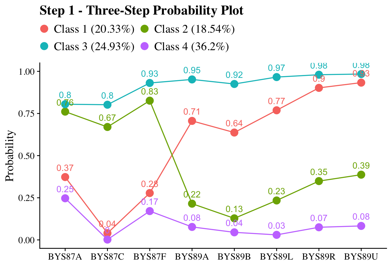
Check that log-likelihood values are the same
output_one <- readModels(here("29-dang-lca-example", "three_step", "one.out"))
output_one$summaries$LL
#> [1] -45812.59

enumeration_c5 <- readModels(here("29-dang-lca-example", "enumeration", "c4_math_weighted.out"))
enumeration_c5$summaries$LL
#> [1] -45812.59
28.5.2 Step 2 - Determine Measurement Error
Extract logits for the classification probabilities for the most likely latent class
logit_cprobs <- as.data.frame(output_one$class_counts$logitProbs.mostLikely)
logit_cprobs
#>        1      2      3 4
#> 1  2.691 -0.448 -0.013 0
#> 2 -0.893  1.664 -1.308 0
#> 3  3.261  2.159  5.684 0
#> 4 -3.825 -3.826 -5.953 0
Extract saved dataset from step one
savedata <- as.data.frame(output_one$savedata) %>%
  rename(N = MLCC) #Rename the column in savedata named "MLCC" and change to "N"
Check variable names in savedata (Mplus will cut off variable names that are longer than 8 characters)
names(savedata)
#>  [1] "BYS87A"   "BYS87C"   "BYS87F"   "BYS89A"   "BYS89B"
#>  [6] "BYS89L"   "BYS89R"   "BYS89U"   "FEMALE"   "SES_DICH"
#> [11] "F3ONET2C" "CPROB1"   "CPROB2"   "CPROB3"   "CPROB4"
#> [16] "N"        "F3BYTSCW"
28.5.3 Step 3 - LCA Auxiliary Variable Model with 2 covariates and 1 distal outcome
Model with 1 covariate (FEMALE) and 1 distal outcome (Math IRT scores)
step3  <- mplusObject(
  TITLE = "Step 3 - Three-Step",

  VARIABLE =
 "nominal=N;
  classes = c(4);
  usevar = N FEMALE SES_DICH F3ONET2C;
  categorical = F3ONET2C;" , # Add covariates and distal outcomes in addition to `N` here

  ANALYSIS =
 "estimator = mlr;
  type = mixture;
  starts = 0;",

  DEFINE =
   "center FEMALE SES_DICH (grandmean);",

  MODEL =
  glue(
 " %OVERALL%

  F3ONET2C on FEMALE SES_DICH; ! covariate as a related to the distal outcome
  C on female (f1-f3);
  C on SES_DICH (s1-s3);

     %C#1%
  [n#1@{logit_cprobs[1,1]}]; ! MUST EDIT if you do not have a 5-class model.
  [n#2@{logit_cprobs[1,2]}];
  [n#3@{logit_cprobs[1,3]}];

  [F3ONET2C$1](m1);    ! conditional distal logit

  %C#2%
  [n#1@{logit_cprobs[2,1]}];
  [n#2@{logit_cprobs[2,2]}];
  [n#3@{logit_cprobs[2,3]}];

  [F3ONET2C$1](m2);

  %C#3%
  [n#1@{logit_cprobs[3,1]}];
  [n#2@{logit_cprobs[3,2]}];
  [n#3@{logit_cprobs[3,3]}];

  [F3ONET2C$1](m3);

  %C#4%
  [n#1@{logit_cprobs[4,1]}];
  [n#2@{logit_cprobs[4,2]}];
  [n#3@{logit_cprobs[4,3]}];

  [F3ONET2C$1](m4);

 "),

 MODELCONSTRAINT =
 "New (
    ! Distal mean differences (6 total for 4 classes)
    diff12 diff13 diff14
    diff23 diff24 diff34
  );

  ! Distal mean comparisons
  diff12 = m1-m2;
  diff13 = m1-m3;
  diff14 = m1-m4;
  diff23 = m2-m3;
  diff24 = m2-m4;
  diff34 = m3-m4;
 ",

  MODELTEST = "     ! omnibus test of distal means
    m1=m2;
    m2=m3;
    m3=m4;

    !f1=0;       ! omnibus test of covariate logits (female)
    !f2=0;
    !f3=0;

    !s1=0;       ! omnibus test of covariate logits (ses)
    !s2=0;
    !s3=0;
   ",

 OUTPUT = "sampstat",

  usevariables = colnames(savedata),
  rdata = savedata)

step3_fit <- mplusModeler(step3,
               dataout=here("29-dang-lca-example", "three_step", "Step3.dat"),
               modelout=here("29-dang-lca-example", "three_step", "three_distal.inp"),
               check=TRUE, run = TRUE, hashfilename = FALSE)
Rerun model with different model test:
# Update the model test by overwriting string
step3$MODELTEST <- "f1=0; f2=0; f3=0;"

# Then run it again
mplusModeler(step3,
               dataout=here("29-dang-lca-example", "three_step", "Step3.dat"),
               modelout=here("29-dang-lca-example", "three_step", "three_female.inp"),
               check=TRUE, run = TRUE, hashfilename = FALSE)
Rerun model with different model test:
# Update the model test by overwriting string
step3$MODELTEST <- "s1=0; s2=0; s3=0;"

# Then run it again
mplusModeler(step3,
               dataout=here("29-dang-lca-example", "three_step", "Step3.dat"),
               modelout=here("29-dang-lca-example", "three_step", "three_ses.inp"),
               check=TRUE, run = TRUE, hashfilename = FALSE)
Compare Step 1 classes and Step 3 classes
output_one <- readModels(here("29-dang-lca-example", "three_step", "one.out"))
output_one$class_counts$modelEstimated
#>   class    count proportion
#> 1     1 2468.993    0.20328
#> 2     2 2252.181    0.18543
#> 3     3 3028.463    0.24934
#> 4     4 4396.363    0.36196


output_three <- readModels(here("29-dang-lca-example", "three_step", "three_distal.out"))
output_three$class_counts$modelEstimated
#>   class    count proportion
#> 1     1 2325.724    0.19148
#> 2     2 2357.554    0.19410
#> 3     3 3066.438    0.25246
#> 4     4 4396.284    0.36195
NOTE: If there are notable differences between class formation in the Step 1 and the Step 3 models, it means there are one of more covariates included in the Step 3 model that may be sources of unaccounted-for DIF
28.6 Visualizations
28.6.0.1 Wald Test Table
This is testing if there is a relation between the latent class variable and the distal outcome.
Note: There are two outputs, each containing separate Wald tests (one for Math IRT scores and the other for self-reported gender). However, other than the Wald test, the outputs are identical. Either can be used for subsequent code.
# Make a Wald table function
wald_table <- function(mplus_model, table_title) {

  # Read the model
  model_output <- mplus_model

  # Extract information as data frame
  wald <- as.data.frame(model_output[["summaries"]]) %>%
    dplyr::select(WaldChiSq_Value:WaldChiSq_PValue) %>%
    mutate(WaldChiSq_DF = paste0("(", WaldChiSq_DF, ")")) %>%
    unite(wald_test, WaldChiSq_Value, WaldChiSq_DF, sep = " ") %>%
    rename(pval = WaldChiSq_PValue) %>%
    mutate(pval = ifelse(pval<0.001, paste0("<.001*"),
                       ifelse(pval<0.05, paste0(scales::number(pval, accuracy = .001), "*"),
                              scales::number(pval, accuracy = .001))))

  # Create the gt table
  wald %>%
  gt() %>%
    tab_header(
    title = table_title) %>%
    cols_label(
      wald_test = md("Wald Test (*df*)"),
      pval = md("*p*-value")) %>%
  cols_align(align = "center") %>%
  opt_align_table_header(align = "left") %>%
  gt::tab_options(table.font.names = "serif")
}
Use wald_table funtion
output_three_distal <- readModels(here("29-dang-lca-example", "three_step", "three_distal.out"))
output_three_female <- readModels(here("29-dang-lca-example", "three_step", "three_female.out"))
output_three_ses <- readModels(here("29-dang-lca-example", "three_step", "three_ses.out"))

wald_table(output_three_distal, "Wald Test Distal Means (Math IRT Scores)")| Wald Test Distal Means (Math IRT Scores) | |
| Wald Test (df) | p-value |
|---|---|
| 39.126 (3) | <.001* |
wald_table(output_three_female, "Wald Test Distal Means (Female)")| Wald Test Distal Means (Female) | |
| Wald Test (df) | p-value |
|---|---|
| 171.432 (3) | <.001* |
wald_table(output_three_ses, "Wald Test Distal Means (SES)")| Wald Test Distal Means (SES) | |
| Wald Test (df) | p-value |
|---|---|
| 120.158 (3) | <.001* |
Note: There are two outputs, each containing separate Wald tests (one for Math IRT scores and the other for self-reported gender). However, other than the Wald test, the outputs are identical. Either can be used for subsequent code.
28.6.0.2 Table of Covariates Relations
Make predictor_table function
# Make a predictor table function
predictor_table <- function(mplus_output,
                            var_labels = NULL,
                            table_title = "Predictors of Class Membership") {

  # Extract Unstandardized Logits
cov_data <- as.data.frame(mplus_output[["parameters"]][["unstandardized"]]) %>%
  filter(str_detect(paramHeader, "\\.ON$")) %>%
  filter(!str_detect(LatentClass, "Categorical\\.Latent\\.Variables")) %>%
  mutate(
    param_label = if (!is.null(var_labels)) {
      str_replace_all(param, var_labels)
    } else {
      str_to_title(param)
    },
    latent_class = paste("Class", LatentClass)
  ) %>%
  mutate(
    logit = paste0(format(round(est, 3), nsmall = 3), " (", format(round(se, 2), nsmall = 2), ")"),
    pval_label = case_when(
      pval < 0.001 ~ "<.001*",
      pval < 0.05  ~ paste0(scales::number(pval, accuracy = .001), "*"),
      TRUE         ~ scales::number(pval, accuracy = .001)
    )
  ) %>%
  dplyr::select(param_label, latent_class, logit, pval_label)

  # Extract Odds Ratios
  or_data <- as.data.frame(mplus_output[["parameters"]][["odds"]]) %>%
    filter(str_detect(paramHeader, "\\.ON$")) %>%
    mutate(
      param_label = if (!is.null(var_labels)) {
        str_replace_all(param, var_labels)
      } else {
        str_to_title(param)
      },

      latent_class = paste("Class", LatentClass),

      CI = paste0("[", format(round(lower_2.5ci, 3), nsmall = 3), ", ",
                  format(round(upper_2.5ci, 3), nsmall = 3), "]")
    ) %>%
    dplyr::select(param_label, latent_class, or = est, CI)

  # Combine and Format Table
  or_data %>%
    full_join(cov_data, by = c("param_label", "latent_class")) %>%
    dplyr::select(param_label, latent_class, logit, pval_label, or, CI) %>%
    gt(groupname_col = "latent_class", rowname_col = "param_label") %>%
    tab_header(title = table_title) %>%
    cols_label(
      logit = md("Logit (*se*)"),
      or = md("Odds Ratio"),
      CI = md("95% CI"),
      pval_label = md("*p*-value")
    ) %>%
    sub_missing(missing_text = "-") %>%
    cols_align(align = "center") %>%
    opt_align_table_header(align = "left") %>%
    gt::tab_options(table.font.names = "serif")
}
Use predictor_table function
output_three <- readModels(here("29-dang-lca-example", "three_step", "three_distal.out"))
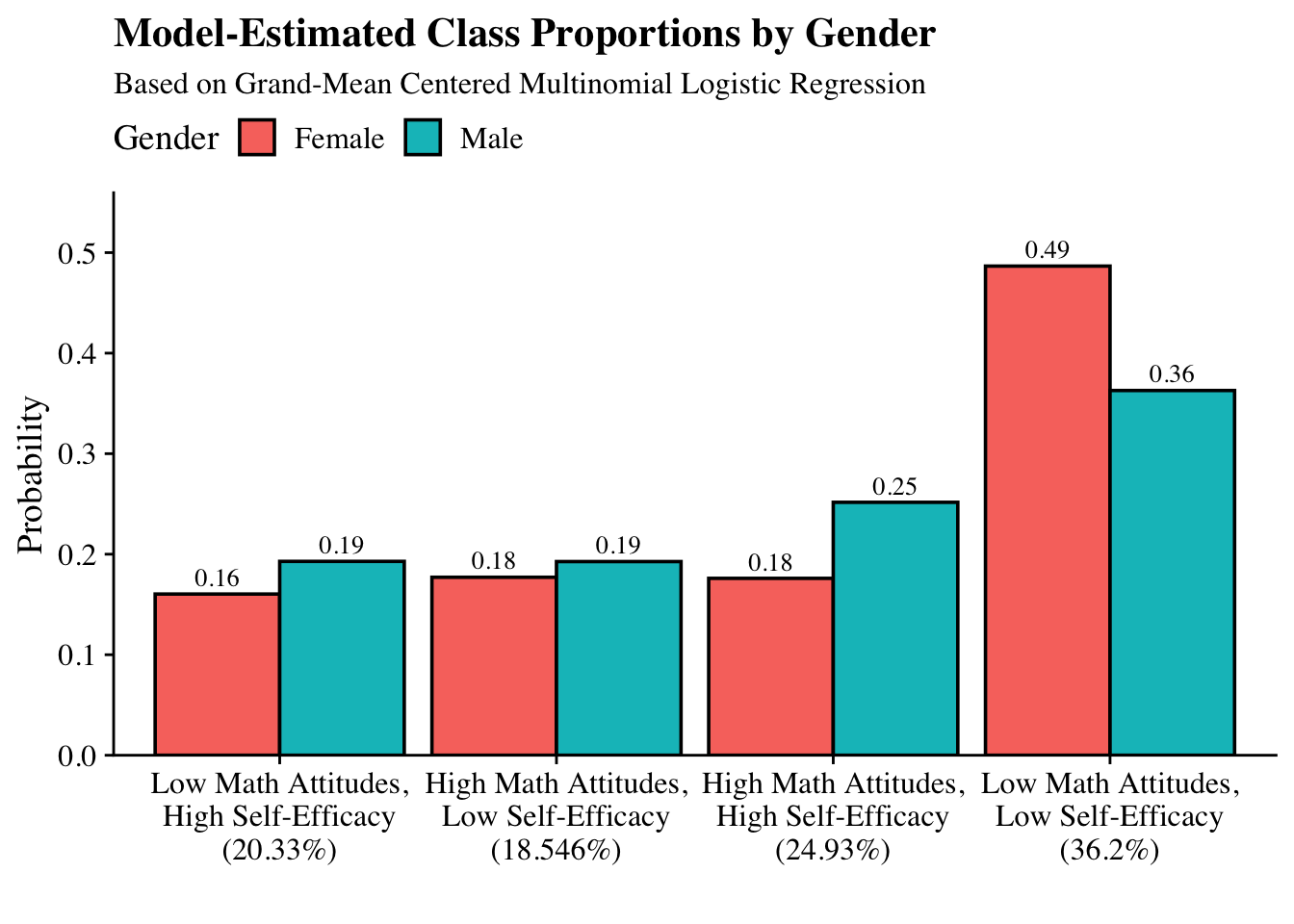
predictor_table(output_three, var_labels = c("FEMALE" = "Female", "SES_DICH" = "SES"))28.6.0.3 Plot of Gender Differences
Class 1 = Low Math Attitudes, High Self-Efficacy (20.33%) Class 2 = High Math Attitudes, Low Self-Efficacy (18.546%) Class 3 = High Math Attitudes, High Self-Efficacy (24.93%) Class 4 = Low Math Attitudes, Low Self-Efficacy (36.2%)
output_three <- readModels(here("29-dang-lca-example", "three_step", "three_distal.out"))

# Extract Centering Values from Univariate Stats
# These are the values Mplus used for the 'Female' variable after centering
female_x   <- savedata %>% summarize(max_val = max(FEMALE, na.rm = TRUE)) %>% pull(max_val)
male_x <- savedata %>% summarize(min_val = min(FEMALE, na.rm = TRUE)) %>% pull(min_val)

# Extract Intercepts and Slopes from Parameters
params <- as.data.frame(output_three$parameters$unstandardized)

# Get Intercepts (C#1 to C#4)
intercepts <- params %>%
  filter(paramHeader == "Intercepts" & str_detect(param, "C#")) %>%
  mutate(Class = as.numeric(str_extract(param, "\\d+"))) %>%
  select(Class, intercept = est)

# Get Slopes (C#1.ON to C#4.ON)
slopes <- params %>%
  filter(str_detect(paramHeader, "C#\\d+\\.ON") & param == "FEMALE") %>%
  mutate(Class = as.numeric(str_extract(paramHeader, "\\d+"))) %>%
  select(Class, slope = est)

# Merge and add the Reference Class (Class 4), which is fixed to 0 in your model
logits_df <- full_join(intercepts, slopes, by = "Class") %>%
  add_row(Class = 4, intercept = 0, slope = 0) %>%
  arrange(Class)

# Class labels
class_labels <- c("1" = "Low Math Attitudes, High Self-Efficacy (20.33%)",
                  "2" = "High Math Attitudes, Low Self-Efficacy (18.546%)",
                  "3" = "High Math Attitudes, High Self-Efficacy (24.93%)",
                  "4" = "Low Math Attitudes, Low Self-Efficacy (36.2%)")

# Calculate Predicted Probabilities
plot_data <- logits_df %>%
  # Create a row for each gender within each class
  crossing(Gender = c("Male", "Female")) %>%
  mutate(
    # Use centered values: Male (-0.485) and Female (0.515)
    x_val = ifelse(Gender == "Male", male_x, female_x),
    logit = intercept + (slope * x_val)
  ) %>%
  group_by(Gender) %>%
  mutate(
    # Apply Softmax: P = exp(logit) / sum(exp(logits))
    prob = exp(logit) / sum(exp(logit)),
    Class_Name = str_wrap(class_labels[as.character(Class)], width = 20)
  )

# Generate the Plot
ggplot(plot_data, aes(x = fct_inorder(Class_Name), y = prob, fill = Gender)) +
  geom_bar(stat = "identity", position = position_dodge(width = 0.9), color = "black") +
  geom_text(aes(label = sprintf("%.2f", prob)),
            position = position_dodge(width = 0.9),
            vjust = -0.5, size = 3.5, family = "serif") +
  scale_y_continuous(expand = expansion(mult = c(0, 0.15))) +
  labs(
    title = "Model-Estimated Class Proportions by Gender",
    subtitle = "Based on Grand-Mean Centered Multinomial Logistic Regression",
    x = "",
    y = "Probability",
    fill = "Gender"
  ) +
  theme_cowplot() +
  theme(
    text = element_text(family = "serif"),
    panel.grid.major.x = element_blank(),
    legend.position = "top"
  )
28.6.0.4 Plot of SES Differences
output_three <- readModels(here("29-dang-lca-example", "three_step", "three_distal.out"))
# Extract Centering Values from Univariate Stats
# These are the values Mplus used for the 'Female' variable after centering
low_ses_x <- savedata %>% summarize(max_val = max(SES_DICH, na.rm = TRUE)) %>% pull(max_val)
other_ses_x <- savedata %>% summarize(min_val = min(SES_DICH, na.rm = TRUE)) %>% pull(min_val)
# Extract Intercepts and Slopes from Parameters
params <- as.data.frame(output_three$parameters$unstandardized)
# Get Intercepts (C#1 to C#4)
intercepts <- params %>%
filter(paramHeader == "Intercepts" & str_detect(param, "C#")) %>%
mutate(Class = as.numeric(str_extract(param, "\\d+"))) %>%
select(Class, intercept = est)
# Get Slopes (C#1.ON to C#4.ON)
slopes <- params %>%
filter(str_detect(paramHeader, "C#\\d+\\.ON") & param == "SES_DICH") %>%
mutate(Class = as.numeric(str_extract(paramHeader, "\\d+"))) %>%
select(Class, slope = est)
# Merge and add the Reference Class (Class 5), which is fixed to 0 in your model
logits_df <- full_join(intercepts, slopes, by = "Class") %>%
add_row(Class = 4, intercept = 0, slope = 0) %>%
arrange(Class)
# Class labels
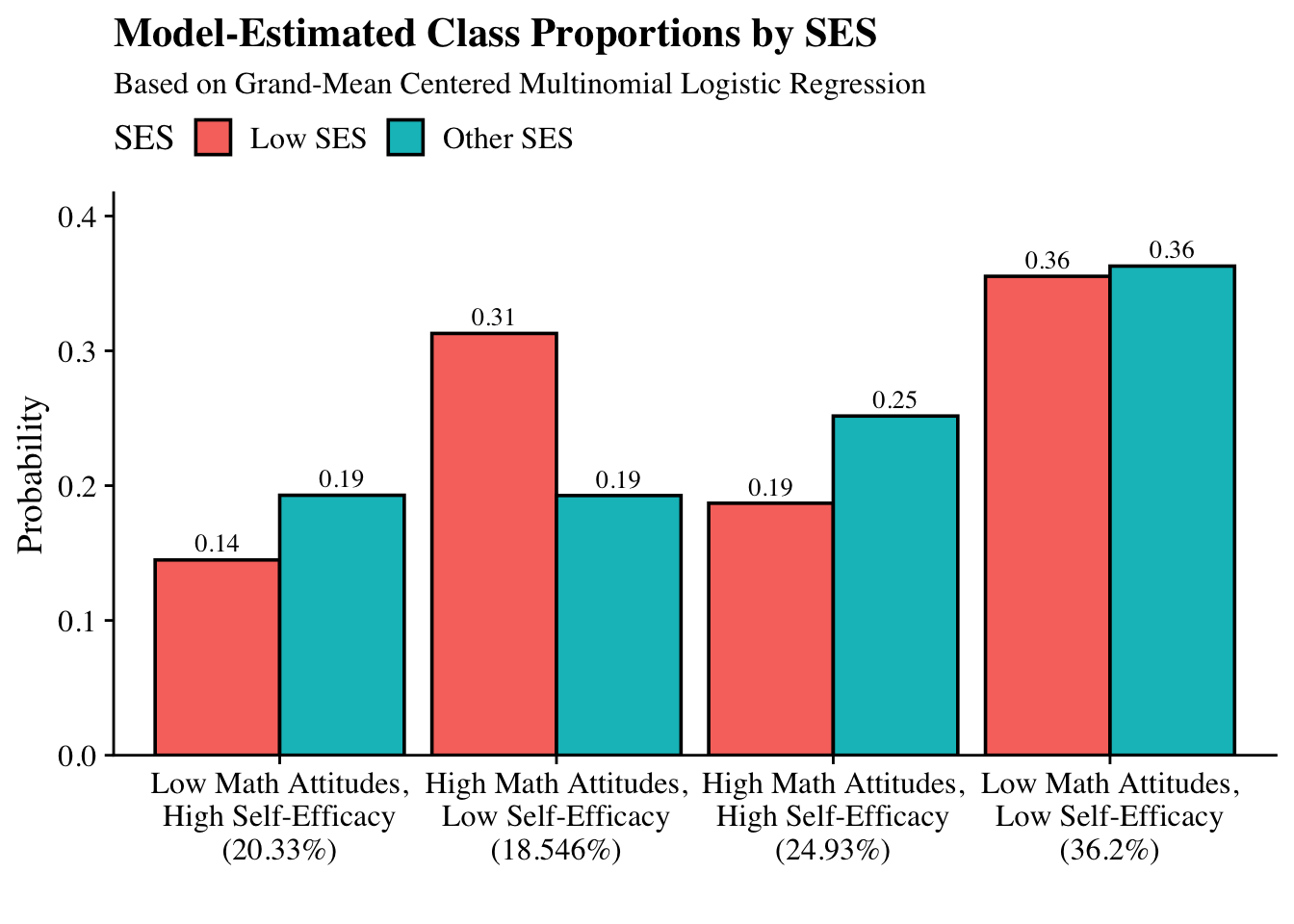
class_labels <- c("1" = "Low Math Attitudes, High Self-Efficacy (20.33%)",
"2" = "High Math Attitudes, Low Self-Efficacy (18.546%)",
"3" = "High Math Attitudes, High Self-Efficacy (24.93%)",
"4" = "Low Math Attitudes, Low Self-Efficacy (36.2%)")
# Calculate Predicted Probabilities
plot_data <- logits_df %>%
# Create a row for each gender within each class
crossing(SES = c("Other SES", "Low SES")) %>%
mutate(
# Use centered values: Male (-0.485) and Female (0.515)
x_val = ifelse(SES == "Other SES", other_ses_x, low_ses_x),
logit = intercept + (slope * x_val)
) %>%
group_by(SES) %>%
mutate(
# Apply Softmax: P = exp(logit) / sum(exp(logits))
prob = exp(logit) / sum(exp(logit)),
Class_Name = str_wrap(class_labels[as.character(Class)], width = 20)
)
# Generate the Plot
ggplot(plot_data, aes(x = fct_inorder(Class_Name), y = prob, fill = SES)) +
geom_bar(stat = "identity", position = position_dodge(width = 0.9), color = "black") +
geom_text(aes(label = sprintf("%.2f", prob)),
position = position_dodge(width = 0.9),
vjust = -0.5, size = 3.5, family = "serif") +
scale_y_continuous(expand = expansion(mult = c(0, 0.15))) +
labs(
title = "Model-Estimated Class Proportions by SES",
subtitle = "Based on Grand-Mean Centered Multinomial Logistic Regression",
x = "",
y = "Probability",
fill = "SES"
) +
theme_cowplot() +
theme(
text = element_text(family = "serif"),
panel.grid.major.x = element_blank(),
legend.position = "top"
)
28.6.0.5 Table of Pairwise Distal Outcome Differences
Make diff_table function
diff_table <- function(mplus_output,
                       prefix = "DIFF",
                       table_title = "Pairwise Comparisons") {

  # Extract and Clean
  diff_data <- as.data.frame(mplus_output[["parameters"]][["unstandardized"]]) %>%
    # Dynamically filter by the prefix provided (e.g., DIFF or FEM)
    filter(str_detect(param, paste0("^", prefix))) %>%
    dplyr::select(param, est, se, pval) %>%
    # Format Estimate and SE
    mutate(
      estimate = paste0(format(round(est, 3), nsmall = 3),
                        " (", format(round(se, 2), nsmall = 2), ")")
    ) %>%
    # Logic to split "DIFF12" into "1" and "2"
    mutate(
      digits = str_remove(param, prefix),
      Group1 = substr(digits, 1, 1),
      Group2 = substr(digits, 2, 2),
      comparison = paste0("Class ", Group1, " vs. Class ", Group2)
    ) %>%
    # Format p-values
    mutate(pval_label = case_when(
      pval < 0.001 ~ "<.001*",
      pval < 0.05  ~ paste0(scales::number(pval, accuracy = .001), "*"),
      TRUE         ~ scales::number(pval, accuracy = .001)
    )) %>%
    dplyr::select(comparison, estimate, pval_label)

  # Create Table
  diff_data %>%
    gt() %>%
    tab_header(title = table_title) %>%
    cols_label(
      comparison = "Comparison",
      estimate = md("Difference (*se*)"),
      pval_label = md("*p*-value")
    ) %>%
    cols_align(align = "center") %>%
    opt_align_table_header(align = "left") %>%
    gt::tab_options(table.font.names = "serif")
}
Use diff_table function
output_three <- readModels(here("29-dang-lca-example", "three_step", "three_distal.out"))

diff_table(
  mplus_output = output_three,
  prefix = "DIFF",
  table_title = "Pairwise Comparisons of Distal Outcome (STEM Occupation)"
)| Pairwise Comparisons of Distal Outcome (STEM Occupation) | ||
| Comparison | Difference (se) | p-value |
|---|---|---|
| Class 1 vs. Class 2 | -0.037 (0.10) | 0.709 |
| Class 1 vs. Class 3 | 0.296 (0.08) | <.001* |
| Class 1 vs. Class 4 | -0.082 (0.08) | 0.299 |
| Class 2 vs. Class 3 | 0.332 (0.09) | <.001* |
| Class 2 vs. Class 4 | -0.045 (0.09) | 0.601 |
| Class 3 vs. Class 4 | -0.378 (0.06) | <.001* |
28.6.0.6 Plot Distal Outcome Means
output_three <- readModels(here("29-dang-lca-example", "three_step", "three_distal.out"))

plot_data <- data.frame(
  class_w_label = c(
    "Low Math Attitudes,\nHigh Self-Efficacy (20.33%)",
    "High Math Attitudes,\nLow Self-Efficacy (18.55%)",
    "High Math Attitudes,\nHigh Self-Efficacy (24.93%)",
    "Low Math Attitudes,\nLow Self-Efficacy (36.2%)"
  ),
  est = c(24.6, 24.0, 30.5, 23.1)
)

# Plot bar graphs
plot_data %>%
  ggplot(aes(x=class_w_label, y = est, fill = class_w_label)) +
  geom_col(position = "dodge", stat = "identity", color = "black") +
  geom_text(aes(label = paste0(est, "%")),
            family = "serif", size = 4,
            position=position_dodge(.9),
            vjust = 8) +
 # scale_fill_grey(start = .4, end = .7) + # Remove for colorful bars
  labs(y="STEM Occupation", x="",
           title = "Distal Mean Comparision for STEM Occupation") +
  theme_cowplot() +
  theme(text = element_text(family = "serif"),
        legend.position="none")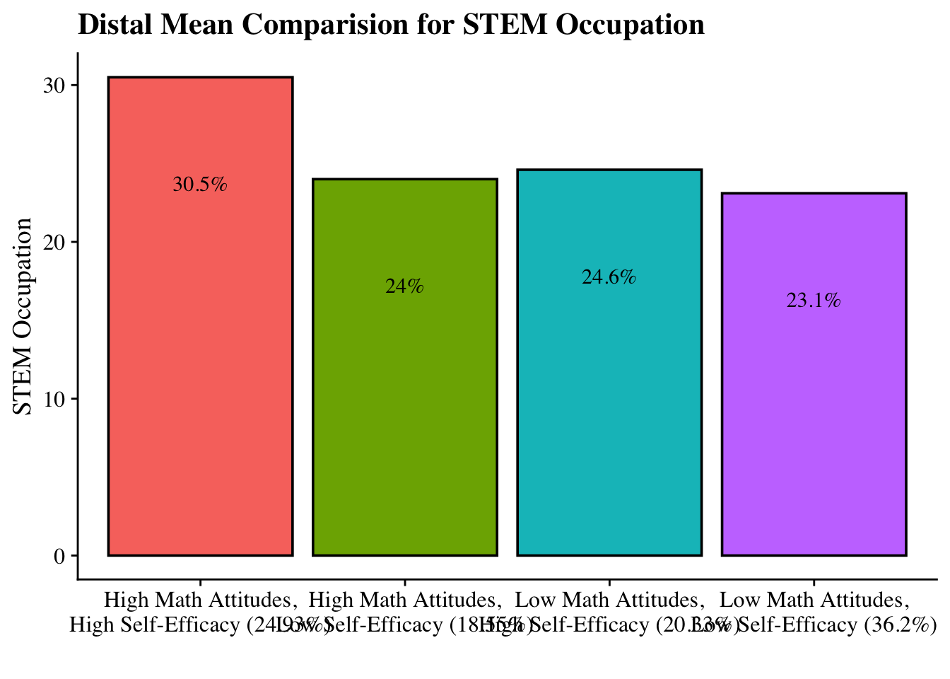
28.6.0.7 Distal outcome regressed on the covariate
Is there a relation between the distal outcome (Math IRT Scores) and the covariate (Gender)?
output_three <- readModels(here("29-dang-lca-example", "three_step", "three_distal.out"))

# Extract information as data frame
donx <- as.data.frame(output_three[["parameters"]][["unstandardized"]]) %>%
  filter(!str_detect(LatentClass, "Categorical\\.Latent\\.Variables")) %>%
  filter(param %in% c("FEMALE", "SES_DICH")) %>%
  mutate(param = str_replace(param, "FEMALE", "Female"),
         param = str_replace(param, "SES_DICH", "SES")) %>%
  mutate(LatentClass = sub("^","Class ", LatentClass)) %>%
  dplyr::select(!paramHeader) %>%
  mutate(se = paste0("(", format(round(se,2), nsmall =2), ")")) %>%
    unite(estimate, est, se, sep = " ") %>%
  dplyr::select(param, estimate, pval) %>%
  distinct(param, .keep_all=TRUE) %>%
  mutate(pval = ifelse(pval<0.001, paste0("<.001*"),
                       ifelse(pval<0.05, paste0(scales::number(pval, accuracy = .001), "*"),
                              scales::number(pval, accuracy = .001))))

# Create table
donx %>%
  gt(groupname_col = "LatentClass", rowname_col = "param") %>%
  tab_header(
    title = "Covariates Predicting STEM Occupation") %>%
  cols_label(
    estimate = md("Estimate (*se*)"),
    pval = md("*p*-value")) %>%
  sub_missing(1:3,
              missing_text = "") %>%
  sub_values(values = c("999.000"), replacement = "-") %>%
  cols_align(align = "center") %>%
  opt_align_table_header(align = "left") %>%
gt::tab_options(table.font.names = "serif")| Covariates Predicting STEM Occupation | ||
| Estimate (se) | p-value | |
|---|---|---|
| Female | -0.221 (0.05) | <.001* |
| SES | -0.336 (0.06) | <.001* |

<<<<<<<< HEAD:31-lta-three-timepoint.Rmd <<<<<<<< HEAD:31-lta-three-timepoint.Rmd # A demonstration of the ML 3-step and BCH in Mplus (Nylund-Gibson, K., Arch, D. N., & Carter, D., 2026) ======== # Nylund-Gibson, K., Arch, D. N., & Carter, D. (2026) >>>>>>>> b52a7ad760959260c2954fae4fe7f361c4713df2:30-lta-three-timepoint.Rmd ======== # Nylund-Gibson, K., Arch, D. N., & Carter, D. (2026) >>>>>>>> b52a7ad760959260c2954fae4fe7f361c4713df2:30-lta-three-timepoint.Rmd
Nylund-Gibson, K., Arch, D. N., & Carter, D. (2026). Latent transition analysis with auxiliary variables: A demonstration of the ML 3-step and BCH in Mplus. The Quantitative Methods for Psychology, 22(1), 1–8. doi: 10.20982/tqmp.22.1.p001.
28.7 Introduction
This R Markdown document accompanies the tutorial manuscript Latent Transition Analysis with Auxiliary Variables: A Demonstration of the ML 3-Step and BCH Methods in Mplus using data from the Longitudinal Study of American Youth (LSAY). Its purpose is to provide a fully reproducible, step-by-step implementation of the multi-step LTA workflow described in the paper using Mplus and the MplusAutomation package in R.
The focus of this document is operational rather than conceptual.
Before estimating the latent class structure, we begin by loading the necessary packages and preparing the dataset to ensure the indicators and sample structure are ready for LTA.
28.8 Data Setup and Preparation
28.8.1 Load Required Packages
# Installation required when using Mplus version 8.6
# devtools::install_github("michaelhallquist/MplusAutomation")
#if (!requireNamespace("BiocManager", quietly = TRUE))
# install.packages("BiocManager")
#BiocManager::install("rhdf5")

library(MplusAutomation)
library(rhdf5)
library(tidyverse)
library(haven)
library(here)
library(glue)
library(janitor)
library(gt)
library(naniar)
library(psych)
library(modelsummary)
library(cowplot)
library(patchwork)28.9 Descriptive Statistics
28.9.1 Indicators
# Define survey questions
all_questions <- c(
  "AB39A", "AB39H", "AB39I", "AB39K", "AB39L", "AB39M", "AB39T", "AB39U", "AB39W", "AB39X", # 7th grade
  "GA32A", "GA32H", "GA32I", "GA32K", "GA32L", "GA33A", "GA33H", "GA33I", "GA33K", "GA33L", # 10th grade
  "KA46A", "KA46H", "KA46I", "KA46K", "KA46L", "KA47A", "KA47H", "KA47I", "KA47K", "KA47L"  # 12th grade
)

# Function to compute stats (count, mean, SD, range)
compute_stats <- function(data, question, grade, question_name) {
  data %>%
    summarise(
      Grade = grade,
      Count = sum(!is.na(.data[[question]])),
      Mean = mean(.data[[question]], na.rm = TRUE),
      SD = sd(.data[[question]], na.rm = TRUE),
      Min = min(.data[[question]], na.rm = TRUE),
      Max = max(.data[[question]], na.rm = TRUE)
    ) %>%
    mutate(Question = question_name)
}

# Define question names and mappings
table_setup <- tibble(
  question_code = all_questions,
  grade = rep(c(7, 10, 12), each = 10),
  question_name = rep(
    c(
      "I enjoy math",
      "Math is useful in everyday problems",
      "Math helps a person think logically",
      "It is important to know math to get a good job",
      "I will use math in many ways as an adult",
      "I enjoy science",
      "Science is useful in everyday problems",
      "Science helps a person think logically",
      "It is important to know science to get a good job",
      "I will use science in many ways as an adult"
    ),
    times = 3
  )
)

# Compute stats for all questions
table1_data <- pmap_dfr(
  list(table_setup$question_code, table_setup$grade, table_setup$question_name),
  ~compute_stats(lsay_data, ..1, ..2, ..3)
) %>%
  mutate(
    Mean = round(Mean, 2),
    SD = round(SD, 2),
    Min = round(Min, 2),
    Max = round(Max, 2)
  ) %>%
  arrange(match(Question, table_setup$question_name), Grade) %>%
  select(Question, Grade, Count, Mean, SD, Min, Max)

# Build table
table1_gt <- table1_data %>%
  gt(groupname_col = "Question") %>%
  tab_header(
    title = "Table 1. Descriptive Statistics for Mathematics and Science Attitudinal Survey Items Included in Analyses"
  ) %>%
  cols_label(
    Grade = "Grade",
    Count = "N",
    Mean = "Prop.",
    SD = "SD",
    Min = "Min",
    Max = "Max"
  ) %>%
  fmt_number(
    columns = c(Mean, SD),
    decimals = 2
  )

# Show table
table1_gt| Table 1. Descriptive Statistics for Mathematics and Science Attitudinal Survey Items Included in Analyses | |||||
| Grade | N | Prop. | SD | Min | Max |
|---|---|---|---|---|---|
| I enjoy math | |||||
| 7 | 1882 | 0.69 | 0.46 | 0 | 1 |
| 10 | 1532 | 0.63 | 0.48 | 0 | 1 |
| 12 | 1120 | 0.57 | 0.50 | 0 | 1 |
| Math is useful in everyday problems | |||||
| 7 | 1851 | 0.72 | 0.45 | 0 | 1 |
| 10 | 1520 | 0.65 | 0.48 | 0 | 1 |
| 12 | 1111 | 0.67 | 0.47 | 0 | 1 |
| Math helps a person think logically | |||||
| 7 | 1847 | 0.65 | 0.48 | 0 | 1 |
| 10 | 1517 | 0.69 | 0.46 | 0 | 1 |
| 12 | 1108 | 0.71 | 0.45 | 0 | 1 |
| It is important to know math to get a good job | |||||
| 7 | 1854 | 0.77 | 0.42 | 0 | 1 |
| 10 | 1517 | 0.68 | 0.47 | 0 | 1 |
| 12 | 1105 | 0.61 | 0.49 | 0 | 1 |
| I will use math in many ways as an adult | |||||
| 7 | 1857 | 0.75 | 0.43 | 0 | 1 |
| 10 | 1525 | 0.65 | 0.48 | 0 | 1 |
| 12 | 1104 | 0.65 | 0.48 | 0 | 1 |
| I enjoy science | |||||
| 7 | 1873 | 0.62 | 0.48 | 0 | 1 |
| 10 | 1526 | 0.59 | 0.49 | 0 | 1 |
| 12 | 1105 | 0.55 | 0.50 | 0 | 1 |
| Science is useful in everyday problems | |||||
| 7 | 1840 | 0.40 | 0.49 | 0 | 1 |
| 10 | 1516 | 0.43 | 0.50 | 0 | 1 |
| 12 | 1099 | 0.48 | 0.50 | 0 | 1 |
| Science helps a person think logically | |||||
| 7 | 1850 | 0.49 | 0.50 | 0 | 1 |
| 10 | 1516 | 0.53 | 0.50 | 0 | 1 |
| 12 | 1100 | 0.56 | 0.50 | 0 | 1 |
| It is important to know science to get a good job | |||||
| 7 | 1857 | 0.40 | 0.49 | 0 | 1 |
| 10 | 1518 | 0.43 | 0.50 | 0 | 1 |
| 12 | 1099 | 0.38 | 0.49 | 0 | 1 |
| I will use science in many ways as an adult | |||||
| 7 | 1873 | 0.46 | 0.50 | 0 | 1 |
| 10 | 1524 | 0.42 | 0.49 | 0 | 1 |
| 12 | 1103 | 0.44 | 0.50 | 0 | 1 |
Data Verification Summary
All attitudinal indicators fall within the expected 0–1 range and show adequate variability across Grades 7, 10, and 12. No recoding or item removal is required before proceeding to enumeration.
28.9.2 Covariates
# Define covariates
covariates <- c(
  "MINORITY", "FEMALE"
)

# Function to compute stats (count, mean, SD, range, % missing)
compute_stats <- function(data, question, question_name) {
  total_n <- nrow(data)
  missing_n <- sum(is.na(data[[question]]))
  percent_missing <- (missing_n / total_n) * 100

  data %>%
    summarise(
      Count = sum(!is.na(.data[[question]])),
      Mean = mean(.data[[question]], na.rm = TRUE),
      SD = sd(.data[[question]], na.rm = TRUE),
      Min = min(.data[[question]], na.rm = TRUE),
      Max = max(.data[[question]], na.rm = TRUE)
    ) %>%
    mutate(
      Question = question_name,
      PercentMissing = round(percent_missing, 2)
    )
}

# Define question names and mappings
table_setup <- tibble(
  question_code = covariates,
  question_name = c(
    "Minority",
    "Gender"
  )
)

# Compute stats for all questions
table1_data <- pmap_dfr(
  list(table_setup$question_code, table_setup$question_name),
  ~compute_stats(lsay_data, ..1, ..2)
) %>%
  mutate(
    Mean = round(Mean, 2),
    SD = round(SD, 2),
    Min = round(Min, 2),
    Max = round(Max, 2)
  ) %>%
  select(Question, Count, PercentMissing, Mean, SD, Min, Max)

# Build table
table1_gt <- table1_data %>%
  gt() %>%
  tab_header(
    title = "Table 1. Descriptive Statistics for Covariates Included in Analyses"
  ) %>%
  cols_label(
    Count = "N",
    PercentMissing = "% Missing",
    Mean = "Mean or Proportion",
    SD = "SD",
    Min = "Min",
    Max = "Max"
  ) %>%
  fmt_number(
    columns = c(PercentMissing, Mean, SD, Min, Max),
    decimals = 2
  )

# Show table
table1_gt| Table 1. Descriptive Statistics for Covariates Included in Analyses | ||||||
| Question | N | % Missing | Mean or Proportion | SD | Min | Max |
|---|---|---|---|---|---|---|
| Minority | 1824 | 4.60 | 0.17 | 0.38 | 0.00 | 1.00 |
| Gender | 1912 | 0.00 | 0.51 | 0.50 | 0.00 | 1.00 |
Data Verification Summary
Covariates show valid ranges, expected missingness patterns, and sufficient variability for use in auxiliary-variable models. All covariates can be included as planned under full-information maximum likelihood.
28.10 Phase 1: Latent Class Enumeration at Each Timepoint (Exploratory Stage)
28.10.1 Time 1 Enumeration (Grade 7)
t1_enum <- lapply(1:6, function(k) {
  enum_t1  <- mplusObject(

   TITLE = glue("Class {k} Time 1"),

   VARIABLE = glue(
    "categorical = AB39A AB39H AB39I AB39K AB39L AB39M AB39T AB39U AB39W AB39X;
     usevar = AB39A AB39H AB39I AB39K AB39L AB39M AB39T AB39U AB39W AB39X;

     classes = c({k});"),

  ANALYSIS =
   "estimator = mlr;
    type = mixture;
    starts = 500 100;
    processors = 12;",

  OUTPUT = "sampstat residual tech11 tech14;",

  usevariables = colnames(lsay_data),
  rdata = lsay_data)

enum_t1_fit <- mplusModeler(enum_t1,
                 dataout=here("three_lta", "phase_1", "t1", "t1.dat"),
                 modelout=glue(here("three_lta", "phase_1", "t1", "c{k}_lca_t1.inp")),
                 check=TRUE, run = TRUE, hashfilename = FALSE)
})
28.10.2 Time 2 Enumeration (Grade 10)
t2_enum <- lapply(1:6, function(k) {
  enum_t2  <- mplusObject(

   TITLE = glue("Class {k} Time 2"),

   VARIABLE = glue(
    "categorical = GA32A GA32H GA32I GA32K GA32L GA33A GA33H GA33I GA33K GA33L;
     usevar = GA32A GA32H GA32I GA32K GA32L GA33A GA33H GA33I GA33K GA33L;

     classes = c({k});"),

  ANALYSIS =
   "estimator = mlr;
    type = mixture;
    starts = 500 100;
    processors = 12;",

  OUTPUT = "sampstat residual tech11 tech14;",

  usevariables = colnames(lsay_data),
  rdata = lsay_data)

enum_t2_fit <- mplusModeler(enum_t2,
                 dataout=here("three_lta", "phase_1", "t2", "t2.dat"),
                 modelout=glue(here("three_lta", "phase_1", "t2", "c{k}_lca_t2.inp")),
                 check=TRUE, run = TRUE, hashfilename = FALSE)
})
28.10.3 Time 3 Enumeration (Grade 12)
t3_enum <- lapply(1:6, function(k) {
  enum_t3  <- mplusObject(

   TITLE = glue("Class {k} Time 3"),

   VARIABLE = glue(
    "categorical = KA46A KA46H KA46I KA46K KA46L KA47A KA47H KA47I KA47K KA47L;
     usevar = KA46A KA46H KA46I KA46K KA46L KA47A KA47H KA47I KA47K KA47L;

     classes = c({k});"),

  ANALYSIS =
   "estimator = mlr;
    type = mixture;
    starts = 500 100;
    processors = 12;",

  OUTPUT = "sampstat residual tech11 tech14;",

  usevariables = colnames(lsay_data),
  rdata = lsay_data)

enum_t3_fit <- mplusModeler(enum_t3,
                 dataout=here("three_lta", "phase_1", "t3", "t3.dat"),
                 modelout=glue(here("three_lta", "phase_1", "t3", "c{k}_lca_t3.inp")),
                 check=TRUE, run = TRUE, hashfilename = FALSE)
})
Enumeration is completed for Grade 12. Agreement in class number and stability across all three waves provides initial empirical support for considering a longitudinal model.
28.11 Extracting and Summarizing Model Fit
28.11.1 Time 1
source(here("functions", "extract_mplus_info.R"))
source(here("functions","enum_table_lca.R"))

# Define the directory where all of the .out files are located.
output_dir <- here("three_lta", "phase_1","t1")

# Get all .out files
output_files <- list.files(output_dir, pattern = "\\.out$", full.names = TRUE)

# Process all .out files into one dataframe
final_data <- map_dfr(output_files, extract_mplus_info_extended)

# Extract Sample_Size from final_data
sample_size <- unique(final_data$Sample_Size)

output_enum_t1 <- readModels(here("three_lta", "phase_1","t1"), quiet = TRUE)

fit_table_lca(output_enum_t1, final_data)| Model Fit Summary Table1 | |||||||||||
| Classes | Par | LL | % Converged | % Replicated |
Model Fit Indices
|
LRTs
|
Smallest Class
|
||||
|---|---|---|---|---|---|---|---|---|---|---|---|
| BIC | aBIC | CAIC | AWE | VLMR | BLRT | n (%) | |||||
| Class 1 Time 1 | 10 | −11,803.43 | 100% | 100% | 23,682.28 | 23,650.51 | 23,692.28 | 23,787.70 | – | – | 1886 (100%) |
| Class 2 Time 1 | 21 | −10,418.76 | 100% | 100% | 20,995.91 | 20,929.19 | 21,016.91 | 21,217.29 | <.001 | <.001 | 782 (41.5%) |
| Class 3 Time 1 | 32 | −10,165.87 | 36% | 100% | 20,573.10 | 20,471.44 | 20,605.10 | 20,910.45 | 0.00 | <.001 | 384 (20.4%) |
| Class 4 Time 1 | 43 | −10,042.97 | 64% | 98% | 20,410.26 | 20,273.64 | 20,453.26 | 20,863.57 | 0.00 | <.001 | 390 (20.7%) |
| Class 5 Time 1 | 54 | −9,969.24 | 66% | 47% | 20,345.76 | 20,174.20 | 20,399.76 | 20,915.04 | 0.04 | <.001 | 175 (9.3%) |
| Class 6 Time 1 | 65 | −9,915.15 | 42% | 67% | 20,320.54 | 20,114.04 | 20,385.54 | 21,005.78 | 0.01 | <.001 | 180 (9.5%) |
| 1 Note. Par = Parameters; LL = model log likelihood; BIC = Bayesian information criterion; aBIC = sample size adjusted BIC; CAIC = consistent Akaike information criterion; AWE = approximate weight of evidence criterion; BLRT = bootstrapped likelihood ratio test p-value; VLMR = Vuong-Lo-Mendell-Rubin adjusted likelihood ratio test p-value; cmPk = approximate correct model probability. | |||||||||||
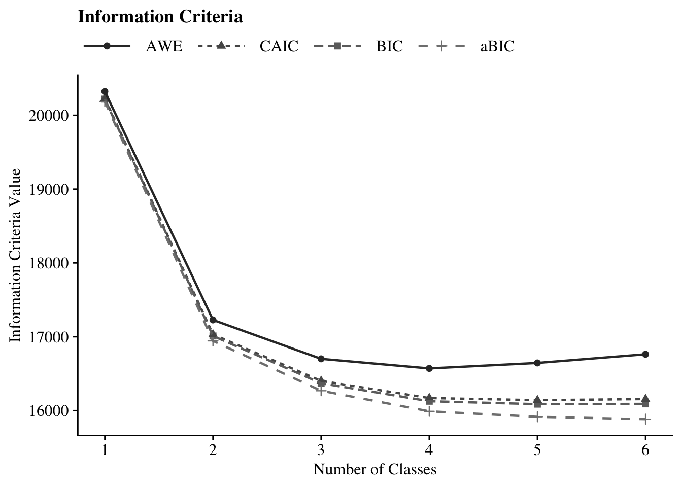
IC Plot
28.11.2 Time 2
# Define the directory where all of the .out files are located.
output_dir <- here("three_lta", "phase_1","t2")

# Get all .out files
output_files <- list.files(output_dir, pattern = "\\.out$", full.names = TRUE)

# Process all .out files into one dataframe
final_data <- map_dfr(output_files, extract_mplus_info_extended)

# Extract Sample_Size from final_data
sample_size <- unique(final_data$Sample_Size)

output_enum_t2 <- readModels(here("three_lta", "phase_1","t2"), quiet = TRUE)
fit_table_lca(output_enum_t2, final_data)| Model Fit Summary Table1 | |||||||||||
| Classes | Par | LL | % Converged | % Replicated |
Model Fit Indices
|
LRTs
|
Smallest Class
|
||||
|---|---|---|---|---|---|---|---|---|---|---|---|
| BIC | aBIC | CAIC | AWE | VLMR | BLRT | n (%) | |||||
| Class 1 Time 2 | 10 | −10,072.93 | 100% | 100% | 20,219.21 | 20,187.44 | 20,229.21 | 20,322.56 | – | – | 1534 (100%) |
| Class 2 Time 2 | 21 | −8,428.38 | 100% | 100% | 17,010.82 | 16,944.10 | 17,031.82 | 17,227.86 | <.001 | <.001 | 658 (42.9%) |
| Class 3 Time 2 | 32 | −8,067.61 | 53% | 100% | 16,369.96 | 16,268.31 | 16,401.96 | 16,700.70 | <.001 | <.001 | 297 (19.4%) |
| Class 4 Time 2 | 43 | −7,905.53 | 39% | 100% | 16,126.50 | 15,989.90 | 16,169.50 | 16,570.93 | <.001 | <.001 | 290 (18.9%) |
| Class 5 Time 2 | 54 | −7,845.44 | 82% | 100% | 16,087.01 | 15,915.46 | 16,141.01 | 16,645.13 | 0.01 | <.001 | 220 (14.3%) |
| Class 6 Time 2 | 65 | −7,806.99 | 44% | 36% | 16,090.79 | 15,884.30 | 16,155.79 | 16,762.61 | 0.02 | <.001 | 130 (8.5%) |
| 1 Note. Par = Parameters; LL = model log likelihood; BIC = Bayesian information criterion; aBIC = sample size adjusted BIC; CAIC = consistent Akaike information criterion; AWE = approximate weight of evidence criterion; BLRT = bootstrapped likelihood ratio test p-value; VLMR = Vuong-Lo-Mendell-Rubin adjusted likelihood ratio test p-value; cmPk = approximate correct model probability. | |||||||||||
IC Plot
28.11.3 Time 3
# Define the directory where all of the .out files are located.
output_dir <- here("three_lta", "phase_1","t3")

# Get all .out files
output_files <- list.files(output_dir, pattern = "\\.out$", full.names = TRUE)

# Process all .out files into one dataframe
final_data <- map_dfr(output_files, extract_mplus_info_extended)

# Extract Sample_Size from final_data
sample_size <- unique(final_data$Sample_Size)

output_enum_t3 <- readModels(here("three_lta", "phase_1","t3"), quiet = TRUE)
fit_table_lca(output_enum_t3, final_data)| Model Fit Summary Table1 | |||||||||||
| Classes | Par | LL | % Converged | % Replicated |
Model Fit Indices
|
LRTs
|
Smallest Class
|
||||
|---|---|---|---|---|---|---|---|---|---|---|---|
| BIC | aBIC | CAIC | AWE | VLMR | BLRT | n (%) | |||||
| Class 1 Time 3 | 10 | −7,349.13 | 100% | 100% | 14,768.49 | 14,736.72 | 14,778.49 | 14,868.72 | – | – | 1122 (100%) |
| Class 2 Time 3 | 21 | −5,976.60 | 100% | 100% | 12,100.68 | 12,033.98 | 12,121.68 | 12,311.16 | <.001 | <.001 | 534 (47.5%) |
| Class 3 Time 3 | 32 | −5,670.60 | 98% | 99% | 11,565.92 | 11,464.28 | 11,597.92 | 11,886.65 | <.001 | <.001 | 203 (18.1%) |
| Class 4 Time 3 | 43 | −5,543.62 | 36% | 97% | 11,389.22 | 11,252.64 | 11,432.22 | 11,820.20 | 0.00 | <.001 | 219 (19.5%) |
| Class 5 Time 3 | 54 | −5,483.67 | 63% | 62% | 11,346.57 | 11,175.06 | 11,400.57 | 11,887.81 | 0.00 | <.001 | 131 (11.7%) |
| Class 6 Time 3 | 65 | −5,444.06 | 42% | 64% | 11,344.60 | 11,138.14 | 11,409.60 | 11,996.08 | 0.09 | <.001 | 81 (7.2%) |
| 1 Note. Par = Parameters; LL = model log likelihood; BIC = Bayesian information criterion; aBIC = sample size adjusted BIC; CAIC = consistent Akaike information criterion; AWE = approximate weight of evidence criterion; BLRT = bootstrapped likelihood ratio test p-value; VLMR = Vuong-Lo-Mendell-Rubin adjusted likelihood ratio test p-value; cmPk = approximate correct model probability. | |||||||||||
IC Plot
28.12 1.5 Plotting Class Probabilities
Plot LCA:
source(here("functions","plot_lca.R"))

step1_t1 <- readModels(here("three_lta", "phase_1","t1"))
step1_t2 <- readModels(here("three_lta", "phase_1","t2"))
step1_t3 <- readModels(here("three_lta", "phase_1","t3"))

t1 <- step1_t1$c4_lca_t1.out
t2 <- step1_t2$c4_lca_t2.out
t3 <- step1_t3$c4_lca_t3.out


(plot_lca(t1) | plot_lca(t2) | plot_lca(t3))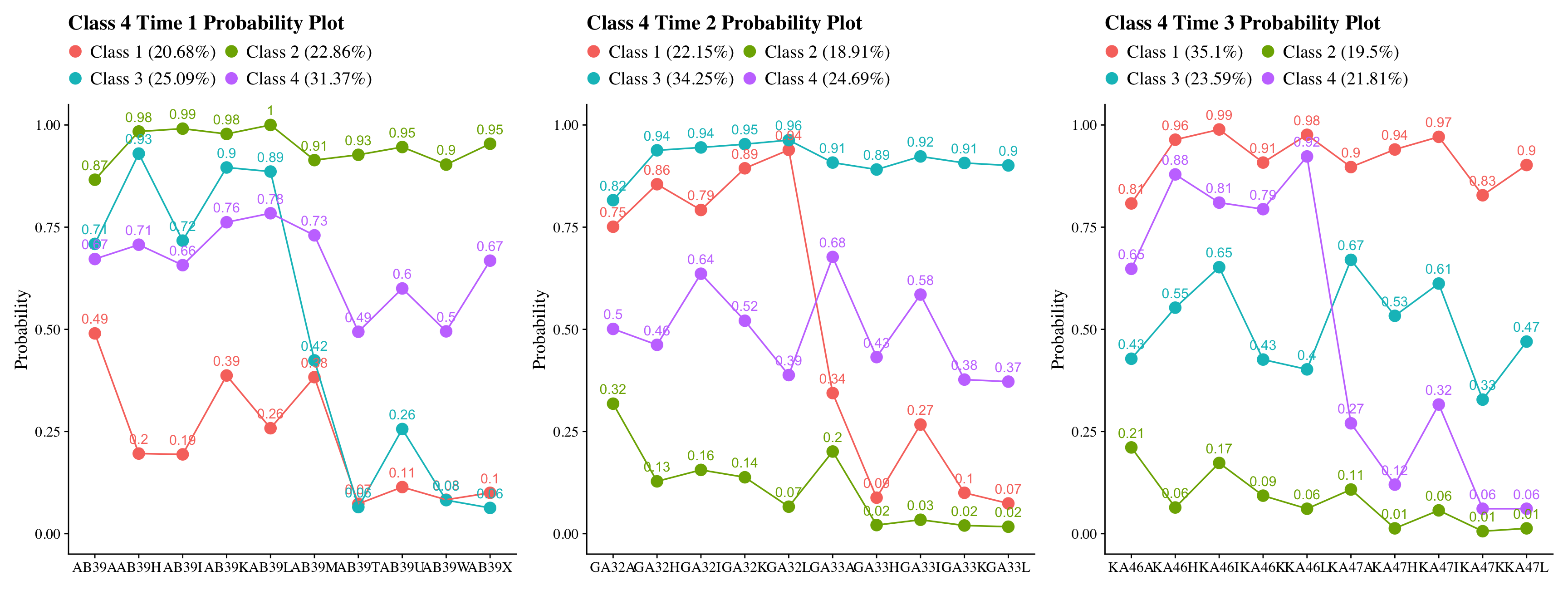
Class labels used here: Class 1: Very Positive, Class 2: Qualified Positive, Class 3: Neutral, Class 4: Less Positive
These diagnostics indicate that the same four-class structure is empirically recoverable across Grades 7, 10, and 12.
28.13 1.6 Estimate LCAs Independently at Each Time Point to Reorder Classes
In this step, the selected four-class solution is re-estimated independently at each wave with:
Fixed number of classes (four)
Optimized class ordering using
optseedSupplied
svalues()to enforce consistent class numbering across wavesRandom starts disabled (
starts = 0)
This step does not change the class structure. Its sole purpose is to ensure stable class labeling across waves prior to joint longitudinal modeling.
28.13.1 Time 1 (Reorder)
lca_t1  <- mplusObject(

  TITLE = "Class-3_Time1",

  VARIABLE =
   "categorical = AB39A AB39H AB39I AB39K AB39L AB39M AB39T AB39U AB39W AB39X;
         usevar = AB39A AB39H AB39I AB39K AB39L AB39M AB39T AB39U AB39W AB39X;
         !useobs = patw2==0;

    classes = c(4);",

  ANALYSIS =
   "estimator = mlr;
    type = mixture;
    starts = 0;
    optseed = 937588;",

  OUTPUT = "TECH1 TECH8 TECH14 svalues(2 3 4 1);",

  usevariables = colnames(lsay_data),
  rdata = lsay_data)


lca_t1_fit <- mplusModeler(lca_t1,
                 dataout=here("three_lta", "phase_1","reordered","t1_lca.dat"),
                 modelout=here("three_lta", "phase_1","reordered","t1_lca_step1.inp"),
                 check=TRUE, run = TRUE, hashfilename = FALSE)
28.13.2 Time 2 (Reorder)
lca_t2  <- mplusObject(

  TITLE = "Class-3_Time2",

  VARIABLE =
   "categorical = GA32A GA32H GA32I GA32K GA32L GA33A GA33H GA33I GA33K GA33L;
         usevar = GA32A GA32H GA32I GA32K GA32L GA33A GA33H GA33I GA33K GA33L;
         !useobs = patw4==0;

    classes = c(4);",

  ANALYSIS =
   "estimator = mlr;
    type = mixture;
    starts = 0;
    optseed = 264935;",

  OUTPUT = "TECH1 TECH8 TECH14 svalues(3 1 4 2);",

  usevariables = colnames(lsay_data),
  rdata = lsay_data)


lca_t2_fit <- mplusModeler(lca_t2,
                 dataout=here("three_lta", "phase_1","reordered","t2_lca.dat"),
                 modelout=here("three_lta", "phase_1","reordered","t2_lca_step1.inp"),
                 check=TRUE, run = TRUE, hashfilename = FALSE)
28.13.3 Time 3 (Reorder)
lca_t3  <- mplusObject(

  TITLE = "Class-3_Time3",

  VARIABLE =
   "categorical = KA46A KA46H KA46I KA46K KA46L KA47A KA47H KA47I KA47K KA47L;
         usevar = KA46A KA46H KA46I KA46K KA46L KA47A KA47H KA47I KA47K KA47L;
         !useobs = patw6==0;

    classes = c(4);",

  ANALYSIS =
   "estimator = mlr;
    type = mixture;
    starts = 0;
    optseed = 366706;",

  OUTPUT = "TECH1 TECH8 TECH14 svalues(1 4 3 2);",

  usevariables = colnames(lsay_data),
  rdata = lsay_data)


lca_t3_fit <- mplusModeler(lca_t3,
                 dataout=here("three_lta", "phase_1","reordered","t3_lca.dat"),
                 modelout=here("three_lta", "phase_1","reordered","t3_lca_step1.inp"),
                 check=TRUE, run = TRUE, hashfilename = FALSE)
28.13.4 Diagnostic Class Plots (Post-Reordering)
source(here("functions","plot_lca.R"))
t1 <- readModels(here("three_lta", "phase_1","reordered","t1_lca_step1.out"))
t2 <- readModels(here("three_lta", "phase_1","reordered","t2_lca_step1.out"))
t3 <- readModels(here("three_lta", "phase_1","reordered","t3_lca_step1.out"))


(plot_lca(t1) | plot_lca(t2) | plot_lca(t3))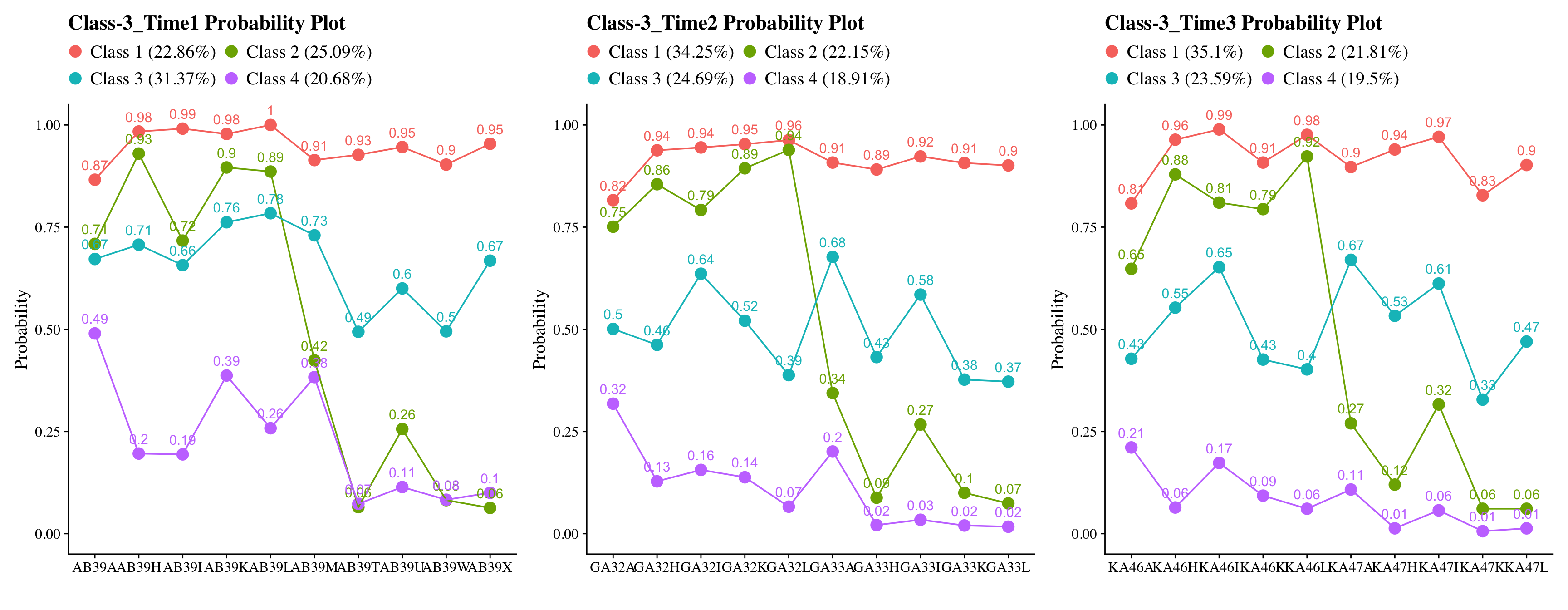
28.14 Phase 2: Testing for Measurement Invariance
28.14.1 Estimate the Non-Invariant Joint Configural Model (No Transitions)
lta_non_inv <- mplusObject(

  TITLE =
    "Non-Invariant LTA Model",

  VARIABLE =
     "idvariable=CASENUM;

      usev =
      AB39A AB39H AB39I AB39K AB39L AB39M AB39T AB39U AB39W AB39X
      GA32A GA32H GA32I GA32K GA32L GA33A GA33H GA33I GA33K GA33L
      KA46A KA46H KA46I KA46K KA46L KA47A KA47H KA47I KA47K KA47L;

      categorical =
      AB39A AB39H AB39I AB39K AB39L AB39M AB39T AB39U AB39W AB39X
      GA32A GA32H GA32I GA32K GA32L GA33A GA33H GA33I GA33K GA33L
      KA46A KA46H KA46I KA46K KA46L KA47A KA47H KA47I KA47K KA47L;

      classes = c1(4) c2(4) c3(4);",

  ANALYSIS =
     "estimator = mlr;
      type = mixture;
      starts = 500 200;",

  MODEL =
     "%overall%

  MODEL c1:
     %c1#1%
     [AB39A$1-AB39X$1];
     %c1#2%
     [AB39A$1-AB39X$1];
     %c1#3%
     [AB39A$1-AB39X$1];
     %c1#4%
     [AB39A$1-AB39X$1];

  MODEL c2:
     %c2#1%
     [GA32A$1-GA33L$1];
     %c2#2%
     [GA32A$1-GA33L$1];
     %c2#3%
     [GA32A$1-GA33L$1];
     %c2#4%
     [GA32A$1-GA33L$1];

  MODEL c3:
     %c3#1%
     [KA46A$1-KA47L$1];
     %c3#2%
     [KA46A$1-KA47L$1];
     %c3#3%
     [KA46A$1-KA47L$1];
     %c3#4%
     [KA46A$1-KA47L$1];",

  OUTPUT = "svalues;",

  usevariables = colnames(lsay_data),
  rdata = lsay_data)

lta_non_inv_fit <- mplusModeler(lta_non_inv,
                     dataout=here("three_lta", "phase_2", "lta.dat"),
                     modelout=here("three_lta", "phase_2", "noninvariant_lta.inp"),
                     check=TRUE, run = TRUE, hashfilename = FALSE)
After estimation, this model is retained strictly as the reference model for nested testing.
28.14.2 Estimate the Full Measurement-Invariance Model
lta_inv <- mplusObject(

  TITLE =
    "Invariant LTA Model",

  VARIABLE =
     "idvariable=CASENUM;

      usev =
      AB39A AB39H AB39I AB39K AB39L AB39M AB39T AB39U AB39W AB39X
      GA32A GA32H GA32I GA32K GA32L GA33A GA33H GA33I GA33K GA33L
      KA46A KA46H KA46I KA46K KA46L KA47A KA47H KA47I KA47K KA47L;

      categorical =
      AB39A AB39H AB39I AB39K AB39L AB39M AB39T AB39U AB39W AB39X
      GA32A GA32H GA32I GA32K GA32L GA33A GA33H GA33I GA33K GA33L
      KA46A KA46H KA46I KA46K KA46L KA47A KA47H KA47I KA47K KA47L;

      classes = c1(4) c2(4) c3(4);",

  ANALYSIS =
     "estimator = mlr;
      type = mixture;
      starts =  0;
      processors=10;",

  MODEL =
     "
     %overall%

  MODEL c1:
     %c1#1%
     [AB39A$1-AB39X$1](1-10);
     %c1#2%
     [AB39A$1-AB39X$1](11-20);
     %c1#3%
     [AB39A$1-AB39X$1](21-30);
     %c1#4%
     [AB39A$1-AB39X$1](31-40);

  MODEL c2:
     %c2#1%
     [GA32A$1-GA33L$1](1-10);
     %c2#2%
     [GA32A$1-GA33L$1](11-20);
     %c2#3%
     [GA32A$1-GA33L$1](21-30);
     %c2#4%
     [GA32A$1-GA33L$1](31-40);

  MODEL c3:
     %c3#1%
     [KA46A$1-KA47L$1](1-10);
     %c3#2%
     [KA46A$1-KA47L$1](11-20);
     %c3#3%
     [KA46A$1-KA47L$1](21-30);
     %c3#4%
     [KA46A$1-KA47L$1](31-40);",

  OUTPUT = "svalues;",

  usevariables = colnames(lsay_data),
  rdata = lsay_data)

lta_inv_fit <- mplusModeler(lta_inv,
                     dataout=here("three_lta", "phase_2", "lta.dat"),
                     modelout=here("three_lta", "phase_2", "invariant_lta.inp"),
                     check=TRUE, run = TRUE, hashfilename = FALSE)
This model yields the measurement structure used for all downstream auxiliary-variable analyses if invariance is retained.
28.14.3 Plotting the Non-Invariant and Invariant Models
source(here("functions","plot_lta.R"))

inv_mod <- readModels(here("three_lta", "phase_2"), quiet = TRUE)

plot_lta(inv_mod$invariant_lta.out)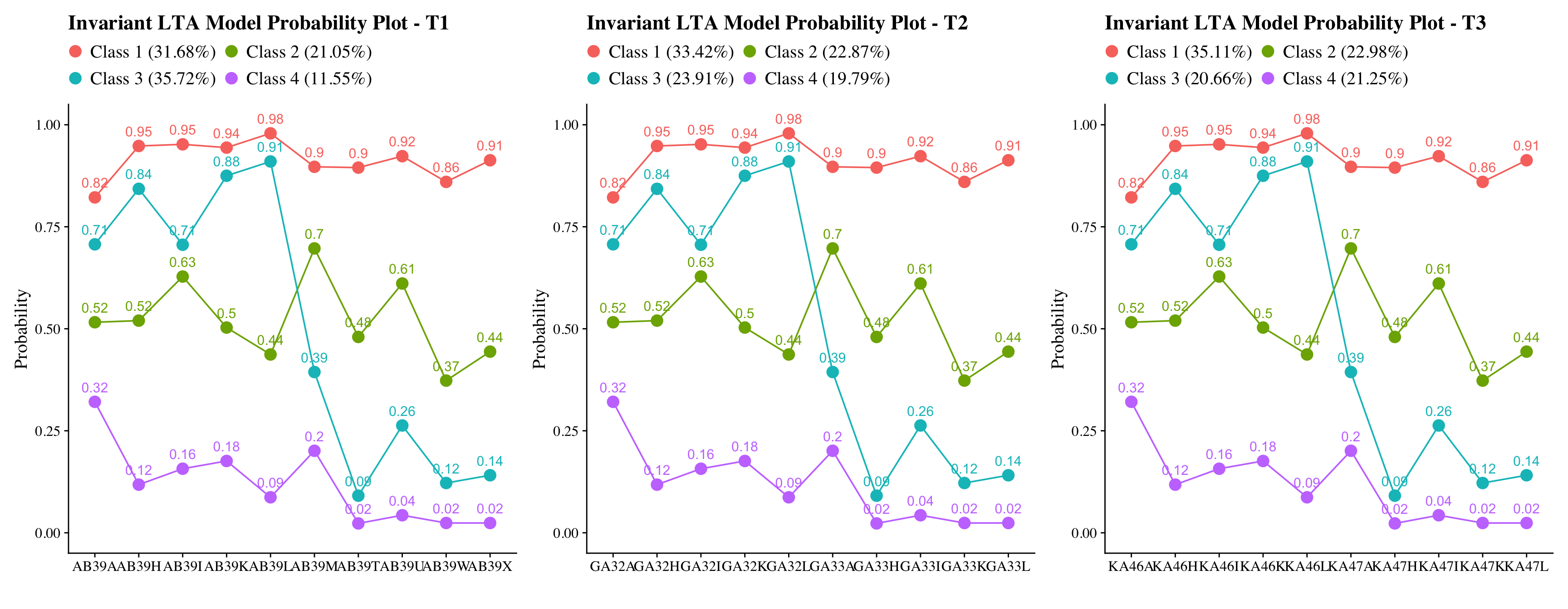
plot_lta(inv_mod$noninvariant_lta.out)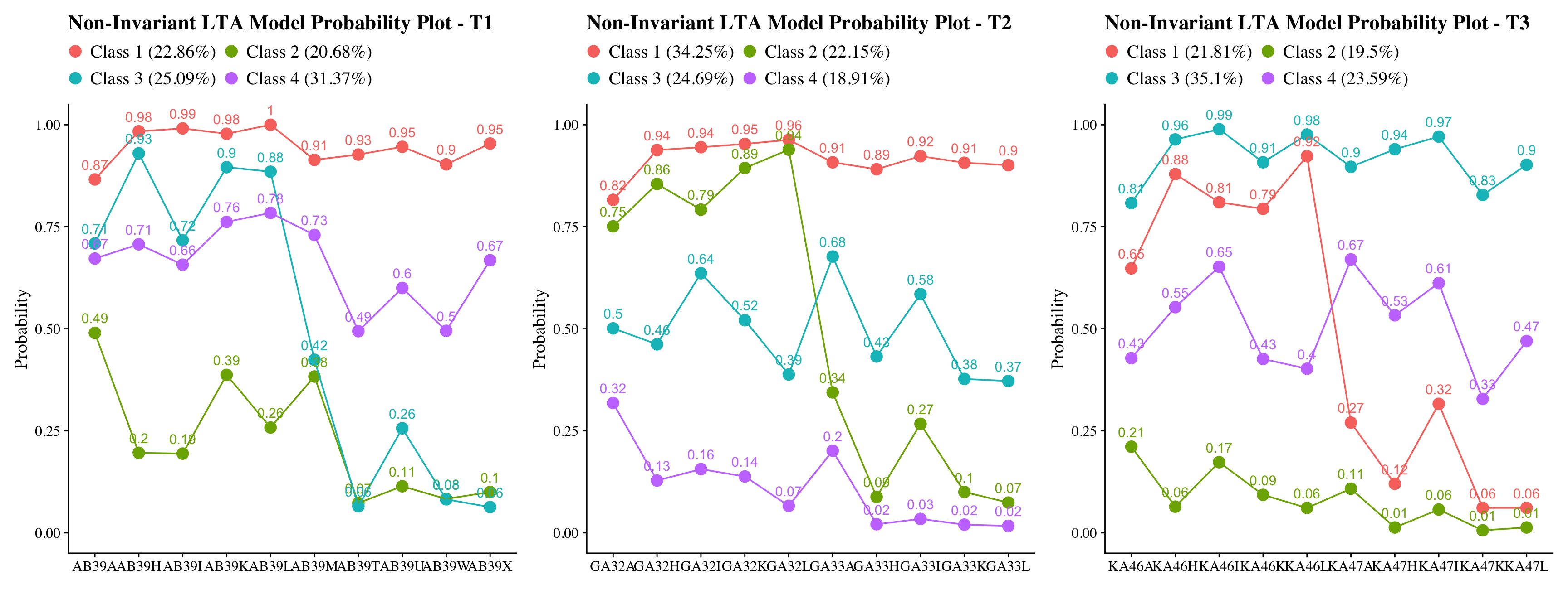
28.15 Nested Model Testing: Satorra–Bentler Scaled χ² Difference Test
# *0 = null or nested model & *1 = comparison  or parent model
lta_models <- readModels(here("three_lta", "phase_2"), quiet = TRUE)

# Log Likelihood Values
L0 <- lta_models$invariant_lta.out$summaries$LL
L1 <- lta_models$noninvariant_lta.out$summaries$LL

# LRT equation
lr <- -2*(L0-L1)

# Parameters
p0 <- lta_models$invariant_lta.out$summaries$Parameters
p1 <- lta_models$noninvariant_lta.out$summaries$Parameters

# Scaling Correction Factors
c0 <- lta_models$invariant_lta.out$summaries$LLCorrectionFactor
c1 <- lta_models$noninvariant_lta.out$summaries$LLCorrectionFactor

# Difference Test Scaling correction
cd <- ((p0*c0)-(p1*c1))/(p0-p1)

# Chi-square difference test(TRd)
TRd <- (lr)/(cd)

# Degrees of freedom
df <- abs(p0 - p1)

# Significance test
(p_diff <- pchisq(TRd, df, lower.tail=FALSE))
#> [1] 2.294394e-40
28.16 Alternatively: Nested Model Testing Using compareModels in MplusAutomation
invisible(capture.output(
  comparison <- compareModels(lta_models$invariant_lta.out, lta_models$noninvariant_lta.out, diffTest=TRUE)
))

# p-value
comparison$diffTest$MLR_LL$p
#> [1] 2.294394e-40

#BIC
comparison$summaries
#>                     Title Observations Estimator Parameters
#> 1     Invariant LTA Model         1907       MLR         49
#> 2 Non-Invariant LTA Model         1907       MLR        129
#>          LL      AIC      BIC
#> 1 -23700.74 47499.48 47771.59
#> 2 -23492.12 47242.24 47958.6228.18 ML Three-Step Procedure
28.18.1 ML STEP 1: Re-Estimate
Time 1: Fixed-Threshold LCA With Saved CPROBS
inv_t1  <- mplusObject(

  TITLE = "Time 1 - Invariant LCA",

  VARIABLE =
   "idvariable=CASENUM;
    categorical = AB39A AB39H AB39I AB39K AB39L AB39M AB39T AB39U AB39W AB39X;
         usevar = AB39A AB39H AB39I AB39K AB39L AB39M AB39T AB39U AB39W AB39X;

    classes = c1(4);

    auxiliary = MINORITY, FEMALE, MATHG7, MATHG10, MATHG12;",

  ANALYSIS =
   "estimator = mlr;
    type = mixture;
    starts = 0;",

  MODEL =
     "%overall%

     %C1#1%

     [ ab39a$1@-1.53313 ] (1);
     [ ab39h$1@-2.90401 ] (2);
     [ ab39i$1@-2.99575 ] (3);
     [ ab39k$1@-2.83359 ] (4);
     [ ab39l$1@-3.85594 ] (5);
     [ ab39m$1@-2.16372 ] (6);
     [ ab39t$1@-2.13876 ] (7);
     [ ab39u$1@-2.48348 ] (8);
     [ ab39w$1@-1.81515 ] (9);
     [ ab39x$1@-2.35163 ] (10);

     %C1#3%

     [ ab39a$1@-0.06349 ] (11);
     [ ab39h$1@-0.07976 ] (12);
     [ ab39i$1@-0.52495 ] (13);
     [ ab39k$1@-0.01216 ] (14);
     [ ab39l$1@0.25484 ] (15);
     [ ab39m$1@-0.83350 ] (16);
     [ ab39t$1@0.07961 ] (17);
     [ ab39u$1@-0.45274 ] (18);
     [ ab39w$1@0.51840 ] (19);
     [ ab39x$1@0.22569 ] (20);

     %C1#2%

     [ ab39a$1@-0.88292 ] (21);
     [ ab39h$1@-1.67761 ] (22);
     [ ab39i$1@-0.87642 ] (23);
     [ ab39k$1@-1.94409 ] (24);
     [ ab39l$1@-2.31259 ] (25);
     [ ab39m$1@0.42887 ] (26);
     [ ab39t$1@2.29606 ] (27);
     [ ab39u$1@1.02908 ] (28);
     [ ab39w$1@1.97179 ] (29);
     [ ab39x$1@1.80988 ] (30);

     %C1#4%

     [ ab39a$1@0.74744 ] (31);
     [ ab39h$1@2.01287 ] (32);
     [ ab39i$1@1.67957 ] (33);
     [ ab39k$1@1.54221 ] (34);
     [ ab39l$1@2.34965 ] (35);
     [ ab39m$1@1.38217 ] (36);
     [ ab39t$1@3.73153 ] (37);
     [ ab39u$1@3.09927 ] (38);
     [ ab39w$1@3.69495 ] (39);
     [ ab39x$1@3.68803 ] (40);",

  OUTPUT = "TECH1 TECH8 TECH14;",

  SAVEDATA =
   "File=t1_inv_cprobs.dat;
    Save=cprob;",

  usevariables = colnames(lsay_data),
  rdata = lsay_data)


inv_t1_fit <- mplusModeler(inv_t1,
                 dataout=here("three_lta", "phase_3","step_1_ml", "t1_inv.dat"),
                 modelout=here("three_lta", "phase_3","step_1_ml", "t1_inv_lca.inp"),
                 check=TRUE, run = TRUE, hashfilename = FALSE)
Time 2: Fixed-Threshold LCA With Saved CPROBS
inv_t2  <- mplusObject(

  TITLE = "Time 2 - Invariant LCA",

  VARIABLE =
   "idvariable=CASENUM;
    categorical = GA32A GA32H GA32I GA32K GA32L GA33A GA33H GA33I GA33K GA33L;
         usevar = GA32A GA32H GA32I GA32K GA32L GA33A GA33H GA33I GA33K GA33L;

    classes = c2(4);

    auxiliary = MINORITY, FEMALE, MATHG7, MATHG10, MATHG12;",

  ANALYSIS =
   "estimator = mlr;
    type = mixture;
    starts = 0;",

  MODEL =
     "%overall%

     %C2#1%

     [ ga32a$1@-1.53313 ] (1);
     [ ga32h$1@-2.90401 ] (2);
     [ ga32i$1@-2.99575 ] (3);
     [ ga32k$1@-2.83359 ] (4);
     [ ga32l$1@-3.85594 ] (5);
     [ ga33a$1@-2.16372 ] (6);
     [ ga33h$1@-2.13876 ] (7);
     [ ga33i$1@-2.48348 ] (8);
     [ ga33k$1@-1.81515 ] (9);
     [ ga33l$1@-2.35163 ] (10);

     %C2#3%

     [ ga32a$1@-0.06349 ] (11);
     [ ga32h$1@-0.07976 ] (12);
     [ ga32i$1@-0.52495 ] (13);
     [ ga32k$1@-0.01216 ] (14);
     [ ga32l$1@0.25484 ] (15);
     [ ga33a$1@-0.83350 ] (16);
     [ ga33h$1@0.07961 ] (17);
     [ ga33i$1@-0.45274 ] (18);
     [ ga33k$1@0.51840 ] (19);
     [ ga33l$1@0.22569 ] (20);

     %C2#2%

     [ ga32a$1@-0.88292 ] (21);
     [ ga32h$1@-1.67761 ] (22);
     [ ga32i$1@-0.87642 ] (23);
     [ ga32k$1@-1.94409 ] (24);
     [ ga32l$1@-2.31259 ] (25);
     [ ga33a$1@0.42887 ] (26);
     [ ga33h$1@2.29606 ] (27);
     [ ga33i$1@1.02908 ] (28);
     [ ga33k$1@1.97179 ] (29);
     [ ga33l$1@1.80988 ] (30);

     %C2#4%

     [ ga32a$1@0.74744 ] (31);
     [ ga32h$1@2.01287 ] (32);
     [ ga32i$1@1.67957 ] (33);
     [ ga32k$1@1.54221 ] (34);
     [ ga32l$1@2.34965 ] (35);
     [ ga33a$1@1.38217 ] (36);
     [ ga33h$1@3.73153 ] (37);
     [ ga33i$1@3.09927 ] (38);
     [ ga33k$1@3.69495 ] (39);
     [ ga33l$1@3.68803 ] (40);
",

  OUTPUT = "TECH1 TECH8 TECH14;",

  SAVEDATA =
   "File=t2_inv_cprobs.dat;
    Save=cprob;",

  usevariables = colnames(lsay_data),
  rdata = lsay_data)


inv_t2_fit <- mplusModeler(inv_t2,
                 dataout=here("three_lta", "phase_3","step_1_ml", "t2_inv.dat"),
                 modelout=here("three_lta", "phase_3","step_1_ml", "t2_inv_lca.inp"),
                 check=TRUE, run = TRUE, hashfilename = FALSE)
Time 3: Fixed-Threshold LCA With Saved CPROBS
inv_t3  <- mplusObject(

  TITLE = "Time 3 - Invariant LCA",

  VARIABLE =
   "idvariable=CASENUM;
    categorical = KA46A KA46H KA46I KA46K KA46L KA47A KA47H KA47I KA47K KA47L;
         usevar = KA46A KA46H KA46I KA46K KA46L KA47A KA47H KA47I KA47K KA47L;

    classes = c3(4);

    auxiliary = MINORITY, FEMALE, MATHG7, MATHG10, MATHG12;",

  ANALYSIS =
   "estimator = mlr;
    type = mixture;
    starts = 0;   ",

    MODEL =
     "%overall%

     %C3#1%

     [ ka46a$1@-1.53313 ] (1);
     [ ka46h$1@-2.90401 ] (2);
     [ ka46i$1@-2.99575 ] (3);
     [ ka46k$1@-2.83359 ] (4);
     [ ka46l$1@-3.85594 ] (5);
     [ ka47a$1@-2.16372 ] (6);
     [ ka47h$1@-2.13876 ] (7);
     [ ka47i$1@-2.48348 ] (8);
     [ ka47k$1@-1.81515 ] (9);
     [ ka47l$1@-2.35163 ] (10);

     %C3#2%

     [ ka46a$1@-0.06349 ] (11);
     [ ka46h$1@-0.07976 ] (12);
     [ ka46i$1@-0.52495 ] (13);
     [ ka46k$1@-0.01216 ] (14);
     [ ka46l$1@0.25484 ] (15);
     [ ka47a$1@-0.83350 ] (16);
     [ ka47h$1@0.07961 ] (17);
     [ ka47i$1@-0.45274 ] (18);
     [ ka47k$1@0.51840 ] (19);
     [ ka47l$1@0.22569 ] (20);

     %C3#3%

     [ ka46a$1@-0.88292 ] (21);
     [ ka46h$1@-1.67761 ] (22);
     [ ka46i$1@-0.87642 ] (23);
     [ ka46k$1@-1.94409 ] (24);
     [ ka46l$1@-2.31259 ] (25);
     [ ka47a$1@0.42887 ] (26);
     [ ka47h$1@2.29606 ] (27);
     [ ka47i$1@1.02908 ] (28);
     [ ka47k$1@1.97179 ] (29);
     [ ka47l$1@1.80988 ] (30);

     %C3#4%

     [ ka46a$1@0.74744 ] (31);
     [ ka46h$1@2.01287 ] (32);
     [ ka46i$1@1.67957 ] (33);
     [ ka46k$1@1.54221 ] (34);
     [ ka46l$1@2.34965 ] (35);
     [ ka47a$1@1.38217 ] (36);
     [ ka47h$1@3.73153 ] (37);
     [ ka47i$1@3.09927 ] (38);
     [ ka47k$1@3.69495 ] (39);
     [ ka47l$1@3.68803 ] (40);",

  OUTPUT = "TECH1 TECH8 TECH14;",

  SAVEDATA =
   "File=t3_inv_cprobs.dat;
    Save=cprob;",

  usevariables = colnames(lsay_data),
  rdata = lsay_data)


inv_t3_fit <- mplusModeler(inv_t3,
                 dataout=here("three_lta", "phase_3","step_1_ml", "t3_inv.dat"),
                 modelout=here("three_lta", "phase_3","step_1_ml", "t3_inv_lca.inp"),
                 check=TRUE, run = TRUE, hashfilename = FALSE)
28.18.1.1 Plotting the Fixed-Threshold LCAs
source(here("functions","plot_lca.R"))

t1 <- readModels(here("three_lta", "phase_3","step_1_ml","t1_inv_lca.out"))
t2 <- readModels(here("three_lta", "phase_3","step_1_ml","t2_inv_lca.out"))
t3 <- readModels(here("three_lta", "phase_3","step_1_ml","t3_inv_lca.out"))

(plot_lca(t1) | plot_lca(t2) | plot_lca(t3))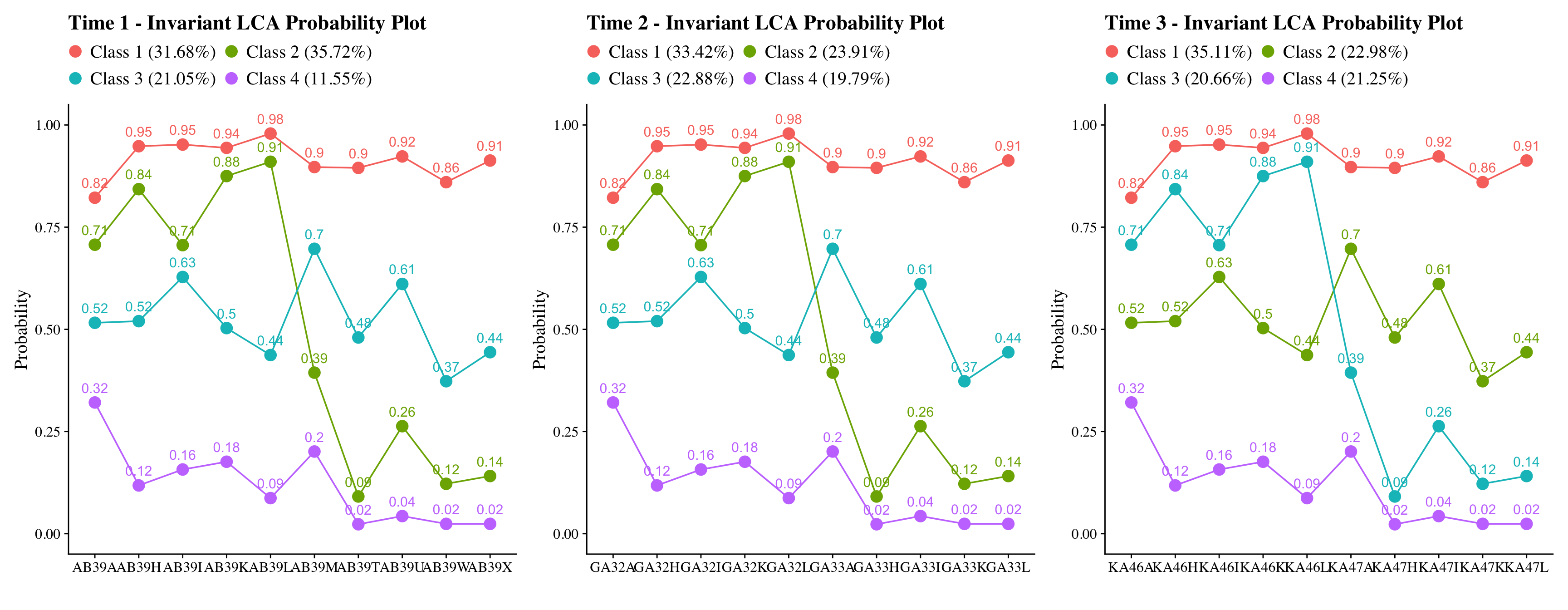
28.18.2 ML STEP 2: Extract Logits and Merge Saved Posterior Data
Extract Classification-Error Logits
inv_step4 <- readModels(here("three_lta", "phase_3","step_1_ml"), quiet = TRUE)

logits_t1 <- as.data.frame(inv_step4$t1_inv_lca.out$class_counts$logitProbs.mostLikely)
logits_t2 <- as.data.frame(inv_step4$t2_inv_lca.out$class_counts$logitProbs.mostLikely)
logits_t3 <- as.data.frame(inv_step4$t3_inv_lca.out$class_counts$logitProbs.mostLikely)
Extract and Merge Saved Posterior Probabilities
savedata_t1 <- as.data.frame(inv_step4$t1_inv_lca.out$savedata) %>%
  rename(cprob11=CPROB1,cprob12=CPROB2,cprob13=CPROB3,cprob14=CPROB4,n1=MLCC1)

savedata_t2 <- as.data.frame(inv_step4$t2_inv_lca.out$savedata) %>%
  rename(cprob21=CPROB1,cprob22=CPROB2,cprob23=CPROB3,cprob24=CPROB4,n2=MLCC2)

savedata_t3 <- as.data.frame(inv_step4$t3_inv_lca.out$savedata) %>%
  rename(cprob31=CPROB1,cprob32=CPROB2,cprob33=CPROB3,cprob34=CPROB4,n3=MLCC3)

savedata_t123 <- savedata_t1 %>%
  full_join(savedata_t2, by = "CASENUM") %>%
  full_join(savedata_t3, by = "CASENUM") %>%
  clean_names() %>% relocate(casenum)

summary(savedata_t123)
#>     casenum         ab39a            ab39h
#>  Min.   :1004   Min.   :0.0000   Min.   :0.0000
#>  1st Qu.:2500   1st Qu.:0.0000   1st Qu.:0.0000
#>  Median :3973   Median :1.0000   Median :1.0000
#>  Mean   :3991   Mean   :0.6881   Mean   :0.7218
#>  3rd Qu.:5505   3rd Qu.:1.0000   3rd Qu.:1.0000
#>  Max.   :6937   Max.   :1.0000   Max.   :1.0000
#>                 NAs    :25       NAs    :56
#>      ab39i           ab39k            ab39l
#>  Min.   :0.000   Min.   :0.0000   Min.   :0.0000
#>  1st Qu.:0.000   1st Qu.:1.0000   1st Qu.:1.0000
#>  Median :1.000   Median :1.0000   Median :1.0000
#>  Mean   :0.653   Mean   :0.7681   Mean   :0.7512
#>  3rd Qu.:1.000   3rd Qu.:1.0000   3rd Qu.:1.0000
#>  Max.   :1.000   Max.   :1.0000   Max.   :1.0000
#>  NAs    :60      NAs    :53       NAs    :50
#>      ab39m            ab39t            ab39u
#>  Min.   :0.0000   Min.   :0.0000   Min.   :0.0000
#>  1st Qu.:0.0000   1st Qu.:0.0000   1st Qu.:0.0000
#>  Median :1.0000   Median :0.0000   Median :0.0000
#>  Mean   :0.6236   Mean   :0.3984   Mean   :0.4924
#>  3rd Qu.:1.0000   3rd Qu.:1.0000   3rd Qu.:1.0000
#>  Max.   :1.0000   Max.   :1.0000   Max.   :1.0000
#>  NAs    :34       NAs    :67       NAs    :57
#>      ab39w            ab39x          minority_x
#>  Min.   :0.0000   Min.   :0.0000   Min.   :0.0000
#>  1st Qu.:0.0000   1st Qu.:0.0000   1st Qu.:0.0000
#>  Median :0.0000   Median :0.0000   Median :0.0000
#>  Mean   :0.3996   Mean   :0.4645   Mean   :0.1704
#>  3rd Qu.:1.0000   3rd Qu.:1.0000   3rd Qu.:0.0000
#>  Max.   :1.0000   Max.   :1.0000   Max.   :1.0000
#>  NAs    :50       NAs    :34       NAs    :105
#>     female_x         mathg7_x       mathg10_x
#>  Min.   :0.0000   Min.   :28.93   Min.   :30.63
#>  1st Qu.:0.0000   1st Qu.:44.84   1st Qu.:58.58
#>  Median :1.0000   Median :53.09   Median :67.71
#>  Mean   :0.5175   Mean   :52.58   Mean   :66.15
#>  3rd Qu.:1.0000   3rd Qu.:59.86   3rd Qu.:75.27
#>  Max.   :1.0000   Max.   :85.07   Max.   :95.26
#>  NAs    :21       NAs    :42      NAs    :532
#>    mathg12_x        cprob11          cprob12
#>  Min.   :27.01   Min.   :0.0000   Min.   :0.0000
#>  1st Qu.:63.40   1st Qu.:0.0000   1st Qu.:0.0030
#>  Median :72.19   Median :0.0080   Median :0.1405
#>  Mean   :71.20   Mean   :0.3169   Mean   :0.3572
#>  3rd Qu.:81.42   3rd Qu.:0.8530   3rd Qu.:0.8210
#>  Max.   :99.30   Max.   :0.9980   Max.   :0.9950
#>  NAs    :1085    NAs    :21       NAs    :21
#>     cprob13          cprob14             n1
#>  Min.   :0.0020   Min.   :0.0000   Min.   :1.000
#>  1st Qu.:0.0090   1st Qu.:0.0000   1st Qu.:1.000
#>  Median :0.0640   Median :0.0000   Median :2.000
#>  Mean   :0.2105   Mean   :0.1155   Mean   :2.093
#>  3rd Qu.:0.2752   3rd Qu.:0.0130   3rd Qu.:3.000
#>  Max.   :0.9990   Max.   :0.9960   Max.   :4.000
#>  NAs    :21       NAs    :21       NAs    :21
#>      ga32a            ga32h            ga32i
#>  Min.   :0.0000   Min.   :0.0000   Min.   :0.0000
#>  1st Qu.:0.0000   1st Qu.:0.0000   1st Qu.:0.0000
#>  Median :1.0000   Median :1.0000   Median :1.0000
#>  Mean   :0.6299   Mean   :0.6493   Mean   :0.6862
#>  3rd Qu.:1.0000   3rd Qu.:1.0000   3rd Qu.:1.0000
#>  Max.   :1.0000   Max.   :1.0000   Max.   :1.0000
#>  NAs    :375      NAs    :387      NAs    :390
#>      ga32k           ga32l            ga33a
#>  Min.   :0.000   Min.   :0.0000   Min.   :0.0000
#>  1st Qu.:0.000   1st Qu.:0.0000   1st Qu.:0.0000
#>  Median :1.000   Median :1.0000   Median :1.0000
#>  Mean   :0.679   Mean   :0.6466   Mean   :0.5917
#>  3rd Qu.:1.000   3rd Qu.:1.0000   3rd Qu.:1.0000
#>  Max.   :1.000   Max.   :1.0000   Max.   :1.0000
#>  NAs    :390     NAs    :382      NAs    :381
#>      ga33h            ga33i            ga33k
#>  Min.   :0.0000   Min.   :0.0000   Min.   :0.0000
#>  1st Qu.:0.0000   1st Qu.:0.0000   1st Qu.:0.0000
#>  Median :0.0000   Median :1.0000   Median :0.0000
#>  Mean   :0.4347   Mean   :0.5251   Mean   :0.4289
#>  3rd Qu.:1.0000   3rd Qu.:1.0000   3rd Qu.:1.0000
#>  Max.   :1.0000   Max.   :1.0000   Max.   :1.0000
#>  NAs    :391      NAs    :391      NAs    :389
#>      ga33l          minority_y        female_y
#>  Min.   :0.0000   Min.   :0.0000   Min.   :0.0000
#>  1st Qu.:0.0000   1st Qu.:0.0000   1st Qu.:0.0000
#>  Median :0.0000   Median :0.0000   Median :1.0000
#>  Mean   :0.4199   Mean   :0.1632   Mean   :0.5254
#>  3rd Qu.:1.0000   3rd Qu.:0.0000   3rd Qu.:1.0000
#>  Max.   :1.0000   Max.   :1.0000   Max.   :1.0000
#>  NAs    :383      NAs    :430      NAs    :373
#>     mathg7_y       mathg10_y       mathg12_y
#>  Min.   :28.93   Min.   :30.63   Min.   :27.01
#>  1st Qu.:46.10   1st Qu.:59.09   1st Qu.:64.00
#>  Median :53.57   Median :67.86   Median :72.56
#>  Mean   :53.20   Mean   :66.41   Mean   :71.63
#>  3rd Qu.:60.09   3rd Qu.:75.30   3rd Qu.:81.73
#>  Max.   :85.07   Max.   :95.26   Max.   :99.30
#>  NAs    :390     NAs    :557     NAs    :1128
#>     cprob21          cprob22          cprob23
#>  Min.   :0.0000   Min.   :0.0000   Min.   :0.0020
#>  1st Qu.:0.0000   1st Qu.:0.0000   1st Qu.:0.0055
#>  Median :0.0035   Median :0.0110   Median :0.0430
#>  Mean   :0.3343   Mean   :0.2391   Mean   :0.2287
#>  3rd Qu.:0.9640   3rd Qu.:0.4000   3rd Qu.:0.3210
#>  Max.   :0.9980   Max.   :0.9920   Max.   :0.9990
#>  NAs    :373      NAs    :373      NAs    :373
#>     cprob24             n2            ka46a
#>  Min.   :0.0000   Min.   :1.000   Min.   :0.000
#>  1st Qu.:0.0000   1st Qu.:1.000   1st Qu.:0.000
#>  Median :0.0000   Median :2.000   Median :1.000
#>  Mean   :0.1979   Mean   :2.275   Mean   :0.567
#>  3rd Qu.:0.1230   3rd Qu.:3.000   3rd Qu.:1.000
#>  Max.   :0.9980   Max.   :4.000   Max.   :1.000
#>  NAs    :373      NAs    :373     NAs    :787
#>      ka46h            ka46i            ka46k
#>  Min.   :0.0000   Min.   :0.0000   Min.   :0.0000
#>  1st Qu.:0.0000   1st Qu.:0.0000   1st Qu.:0.0000
#>  Median :1.0000   Median :1.0000   Median :1.0000
#>  Mean   :0.6733   Mean   :0.7121   Mean   :0.6109
#>  3rd Qu.:1.0000   3rd Qu.:1.0000   3rd Qu.:1.0000
#>  Max.   :1.0000   Max.   :1.0000   Max.   :1.0000
#>  NAs    :796      NAs    :799      NAs    :802
#>      ka46l            ka47a           ka47h
#>  Min.   :0.0000   Min.   :0.000   Min.   :0.000
#>  1st Qu.:0.0000   1st Qu.:0.000   1st Qu.:0.000
#>  Median :1.0000   Median :1.000   Median :0.000
#>  Mean   :0.6513   Mean   :0.552   Mean   :0.485
#>  3rd Qu.:1.0000   3rd Qu.:1.000   3rd Qu.:1.000
#>  Max.   :1.0000   Max.   :1.000   Max.   :1.000
#>  NAs    :803      NAs    :802     NAs    :808
#>      ka47i            ka47k            ka47l
#>  Min.   :0.0000   Min.   :0.0000   Min.   :0.0000
#>  1st Qu.:0.0000   1st Qu.:0.0000   1st Qu.:0.0000
#>  Median :1.0000   Median :0.0000   Median :0.0000
#>  Mean   :0.5645   Mean   :0.3831   Mean   :0.4433
#>  3rd Qu.:1.0000   3rd Qu.:1.0000   3rd Qu.:1.0000
#>  Max.   :1.0000   Max.   :1.0000   Max.   :1.0000
#>  NAs    :807      NAs    :808      NAs    :804
#>     minority          female           mathg7
#>  Min.   :0.0000   Min.   :0.0000   Min.   :28.93
#>  1st Qu.:0.0000   1st Qu.:0.0000   1st Qu.:47.05
#>  Median :0.0000   Median :1.0000   Median :54.23
#>  Mean   :0.1513   Mean   :0.5169   Mean   :54.05
#>  3rd Qu.:0.0000   3rd Qu.:1.0000   3rd Qu.:60.80
#>  Max.   :1.0000   Max.   :1.0000   Max.   :85.07
#>  NAs    :823      NAs    :785      NAs    :793
#>     mathg10         mathg12         cprob31
#>  Min.   :30.63   Min.   :27.01   Min.   :0.0000
#>  1st Qu.:60.66   1st Qu.:63.95   1st Qu.:0.0000
#>  Median :68.83   Median :72.31   Median :0.0060
#>  Mean   :67.49   Mean   :71.59   Mean   :0.3511
#>  3rd Qu.:76.10   3rd Qu.:81.66   3rd Qu.:0.9650
#>  Max.   :95.26   Max.   :99.30   Max.   :0.9980
#>  NAs    :955     NAs    :1137    NAs    :785
#>     cprob32          cprob33          cprob34
#>  Min.   :0.0020   Min.   :0.0000   Min.   :0.0000
#>  1st Qu.:0.0020   1st Qu.:0.0000   1st Qu.:0.0000
#>  Median :0.0400   Median :0.0060   Median :0.0000
#>  Mean   :0.2298   Mean   :0.2066   Mean   :0.2125
#>  3rd Qu.:0.3095   3rd Qu.:0.2480   3rd Qu.:0.2005
#>  Max.   :0.9990   Max.   :0.9910   Max.   :0.9980
#>  NAs    :785      NAs    :785      NAs    :785
#>        n3
#>  Min.   :1.000
#>  1st Qu.:1.000
#>  Median :2.000
#>  Mean   :2.291
#>  3rd Qu.:3.000
#>  Max.   :4.000
#>  NAs    :785
#describe(savedata_t123)
28.18.3 ML STEP 3a: Estimate the Unconditional LTA Model With Fixed Logits
unc_LTA  <- mplusObject(
  TITLE = "Step3a of 3-step",

  VARIABLE =
 "idvariable =casenum;

  nominal=n1 n2 n3;

  usevar = n1 n2 n3;

  classes = c1(4) c2(4) c3(4);

  auxiliary = MINORITY, FEMALE, MATHG7, MATHG10, MATHG12;",

  ANALYSIS =
 "estimator = mlr;
  type = mixture;
  starts = 0;",

  MODEL = glue(
  "%overall%
  c2 on c1;
  c3 on c2;

  Model c1:
    %c1#1%
      [n1#1@{logits_t1[1,1]}];
      [n1#2@{logits_t1[1,2]}];
      [n1#3@{logits_t1[1,3]}];
    %c1#2%
      [n1#1@{logits_t1[2,1]}];
      [n1#2@{logits_t1[2,2]}];
      [n1#3@{logits_t1[2,3]}];
    %c1#3%
      [n1#1@{logits_t1[3,1]}];
      [n1#2@{logits_t1[3,2]}];
      [n1#3@{logits_t1[3,3]}];
    %c1#4%
      [n1#1@{logits_t1[4,1]}];
      [n1#2@{logits_t1[4,2]}];
      [n1#3@{logits_t1[4,3]}];

  Model c2:
    %c2#1%
      [n2#1@{logits_t2[1,1]}];
      [n2#2@{logits_t2[1,2]}];
      [n2#3@{logits_t2[1,3]}];
    %c2#2%
      [n2#1@{logits_t2[2,1]}];
      [n2#2@{logits_t2[2,2]}];
      [n2#3@{logits_t2[2,3]}];
    %c2#3%
      [n2#1@{logits_t2[3,1]}];
      [n2#2@{logits_t2[3,2]}];
      [n2#3@{logits_t2[3,3]}];
    %c2#4%
      [n2#1@{logits_t2[4,1]}];
      [n2#2@{logits_t2[4,2]}];
      [n2#3@{logits_t2[4,3]}];

  Model c3:
    %c3#1%
      [n3#1@{logits_t3[1,1]}];
      [n3#2@{logits_t3[1,2]}];
      [n3#3@{logits_t3[1,3]}];
    %c3#2%
      [n3#1@{logits_t3[2,1]}];
      [n3#2@{logits_t3[2,2]}];
      [n3#3@{logits_t3[2,3]}];
    %c3#3%
      [n3#1@{logits_t3[3,1]}];
      [n3#2@{logits_t3[3,2]}];
      [n3#3@{logits_t3[3,3]}];
    %c3#4%
      [n3#1@{logits_t3[4,1]}];
      [n3#2@{logits_t3[4,2]}];
      [n3#3@{logits_t3[4,3]}];"),

  OUTPUT = "svalues;",

  usevariables = colnames(savedata_t123),
  rdata = savedata_t123)

unc_LTA_fit <- mplusModeler(unc_LTA,
                 dataout=here("three_lta", "phase_3","step_3a_ml", "t123_LTA.dat"),
                 modelout=here("three_lta", "phase_3","step_3a_ml", "unconditional_LTA.inp"),
                 check=TRUE, run = TRUE, hashfilename = FALSE)
28.18.3.1 Plotting Transition Probabilities (Unconditional Model)
source(here("functions","plot_transition.R"))

lta_model <- readModels(here("three_lta", "phase_3","step_3a_ml", "unconditional_LTA.out"))

plot_transition(
  model_name = lta_model,
  facet_labels = c(`1` = "Very Positive", `2` = "Qualified Positive", `3` = "Neutral", `4` = "Less Positive"),
  timepoint_labels = c(`1` = "Grade 7", `2` = "Grade 10", `3` = "Grade 12"),
  class_labels = c(`1` = "Very Positive", `2` = "Qualified Positive", `3` = "Neutral", `4` = "Less Positive")
) +
  labs(title = "Unconditional LTA (ML Three-Step Method)")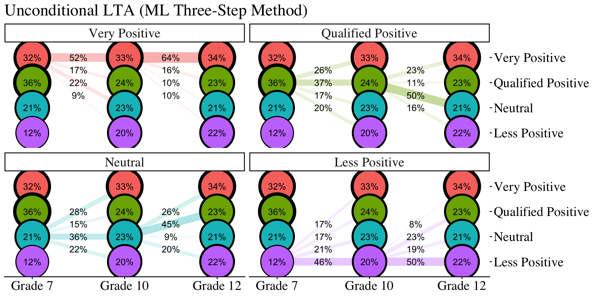
ggsave(here("figures", "unconditional_lta_ml.jpeg"), dpi="retina", height = 6, width = 10, bg = "white", units="in")28.18.4 ML STEP 3b: Estimate the Covariate-Adjusted LTA Model With Fixed Logits
con_LTA  <- mplusObject(
  TITLE = "Step4b of 3-step",

  VARIABLE =
 "idvariable =casenum;

  nominal=n1 n2 n3;

  usevar = n1 n2 n3;

  classes = c1(4) c2(4) c3(4);

  usevar = MINORITY, FEMALE;",

  ANALYSIS =
 "estimator = mlr;
  type = mixture;
  starts = 0;",

  MODEL = glue(
  "%overall%

  c1 ON MINORITY Female;
  c2 ON c1 MINORITY Female;
  c3 ON c2 MINORITY Female;

  Model c1:
    %c1#1%
      [n1#1@{logits_t1[1,1]}];
      [n1#2@{logits_t1[1,2]}];
      [n1#3@{logits_t1[1,3]}];
    %c1#2%
      [n1#1@{logits_t1[2,1]}];
      [n1#2@{logits_t1[2,2]}];
      [n1#3@{logits_t1[2,3]}];
    %c1#3%
      [n1#1@{logits_t1[3,1]}];
      [n1#2@{logits_t1[3,2]}];
      [n1#3@{logits_t1[3,3]}];
    %c1#4%
      [n1#1@{logits_t1[4,1]}];
      [n1#2@{logits_t1[4,2]}];
      [n1#3@{logits_t1[4,3]}];

  Model c2:
    %c2#1%
      [n2#1@{logits_t2[1,1]}];
      [n2#2@{logits_t2[1,2]}];
      [n2#3@{logits_t2[1,3]}];
    %c2#2%
      [n2#1@{logits_t2[2,1]}];
      [n2#2@{logits_t2[2,2]}];
      [n2#3@{logits_t2[2,3]}];
    %c2#3%
      [n2#1@{logits_t2[3,1]}];
      [n2#2@{logits_t2[3,2]}];
      [n2#3@{logits_t2[3,3]}];
    %c2#4%
      [n2#1@{logits_t2[4,1]}];
      [n2#2@{logits_t2[4,2]}];
      [n2#3@{logits_t2[4,3]}];

  Model c3:
    %c3#1%
      [n3#1@{logits_t3[1,1]}];
      [n3#2@{logits_t3[1,2]}];
      [n3#3@{logits_t3[1,3]}];
    %c3#2%
      [n3#1@{logits_t3[2,1]}];
      [n3#2@{logits_t3[2,2]}];
      [n3#3@{logits_t3[2,3]}];
    %c3#3%
      [n3#1@{logits_t3[3,1]}];
      [n3#2@{logits_t3[3,2]}];
      [n3#3@{logits_t3[3,3]}];
    %c3#4%
      [n3#1@{logits_t3[4,1]}];
      [n3#2@{logits_t3[4,2]}];
      [n3#3@{logits_t3[4,3]}];"),

  OUTPUT = "svalues;",

  usevariables = colnames(savedata_t123),
  rdata = savedata_t123)

con_LTA_fit <- mplusModeler(con_LTA,
                 dataout=here("three_lta", "phase_3","step_3b_ml", "t123_LTA.dat"),
                 modelout=here("three_lta", "phase_3","step_3b_ml", "LTA_covariates.inp"),
                 check=TRUE, run = TRUE, hashfilename = FALSE)
28.18.4.1 Covariate Effects Table
lta_cov_model <- readModels(here("three_lta", "phase_3","step_3b_ml", "LTA_covariates.out"))

# REFERENCE CLASS 4
cov <- as.data.frame(lta_cov_model[["parameters"]][["unstandardized"]]) %>%
  filter(param %in% c("MINORITY", "FEMALE")) %>%
  mutate(param = case_when(
            param == "FEMALE" ~ "Gender",
            param == "MINORITY" ~ "URM"),
    se = paste0("(", format(round(se,2), nsmall =2), ")")) %>%
  separate(paramHeader, into = c("Time", "Class"), sep = "#") %>%
  mutate(Class = case_when(
            Class == "1.ON" ~ "Very Positive",
            Class == "2.ON" ~ "Qualified Positive",
            Class == "3.ON" ~ "Neutral"),
         Time = case_when(
            Time == "C1" ~ "7th Grade (T1)",
            Time == "C2" ~ "10th Grade (T2)",
            Time == "C3" ~ "12th Grade (T3)",
         )
         ) %>%
  unite(estimate, est, se, sep = " ") %>%
  select(Time:pval, -est_se) %>%
  mutate(pval = ifelse(pval<0.001, paste0("<.001*"),
                       ifelse(pval<0.05, paste0(scales::number(pval, accuracy = .001), "*"),
                              scales::number(pval, accuracy = .001))))

# Create table

cov_m1 <- cov %>%
  group_by(param, Class) %>%
  gt() %>%
  tab_header(
    title = "Relations Between the Covariates and Latent Class (ML Three-Step Method)") %>%
  tab_footnote(
    footnote = md(
      "Reference Group: Less Positive"
    ),
locations = cells_title()
  ) %>%
  cols_label(
    param = md("Covariate"),
    estimate = md("Estimate (*se*)"),
    pval = md("*p*-value")) %>%
  sub_missing(1:3,
              missing_text = "") %>%
  sub_values(values = c(999.000), replacement = "-") %>%
  cols_align(align = "center") %>%
  opt_align_table_header(align = "left") %>%
  gt::tab_options(table.font.names = "serif")

cov_m1| Relations Between the Covariates and Latent Class (ML Three-Step Method)1 | ||
| Time | Estimate (se) | p-value |
|---|---|---|
| URM - Very Positive | ||
| 7th Grade (T1) | 0.295 (0.40) | 0.459 |
| 10th Grade (T2) | 0.169 (0.33) | 0.611 |
| 12th Grade (T3) | 0.403 (0.37) | 0.273 |
| Gender - Very Positive | ||
| 7th Grade (T1) | -0.398 (0.28) | 0.150 |
| 10th Grade (T2) | -0.124 (0.22) | 0.580 |
| 12th Grade (T3) | 0.155 (0.22) | 0.482 |
| URM - Qualified Positive | ||
| 7th Grade (T1) | -0.174 (0.43) | 0.683 |
| 10th Grade (T2) | 0.429 (0.34) | 0.208 |
| 12th Grade (T3) | 0.818 (0.39) | 0.034* |
| Gender - Qualified Positive | ||
| 7th Grade (T1) | 0.252 (0.29) | 0.380 |
| 10th Grade (T2) | 0.22 (0.25) | 0.379 |
| 12th Grade (T3) | 0.414 (0.26) | 0.105 |
| URM - Neutral | ||
| 7th Grade (T1) | 0.509 (0.47) | 0.279 |
| 10th Grade (T2) | 0.164 (0.39) | 0.673 |
| 12th Grade (T3) | 1.123 (0.40) | 0.005* |
| Gender - Neutral | ||
| 7th Grade (T1) | -0.228 (0.34) | 0.508 |
| 10th Grade (T2) | -0.195 (0.27) | 0.472 |
| 12th Grade (T3) | 0.641 (0.26) | 0.015* |
| 1 Reference Group: Less Positive | ||
28.19 BCH Method
Apply BCH Training Weights for Classification-Error Correction
28.19.1 BCH Step 1: Estimate the Invariant LTA Model and Compute BCH Training Weights
step1_bch  <- mplusObject(
  TITLE = "Step 1 - BCH Method",
  VARIABLE =
     "idvariable=CASENUM;

      usev =
      AB39A AB39H AB39I AB39K AB39L AB39M AB39T AB39U AB39W AB39X
      GA32A GA32H GA32I GA32K GA32L GA33A GA33H GA33I GA33K GA33L
      KA46A KA46H KA46I KA46K KA46L KA47A KA47H KA47I KA47K KA47L;

      categorical =
      AB39A AB39H AB39I AB39K AB39L AB39M AB39T AB39U AB39W AB39X
      GA32A GA32H GA32I GA32K GA32L GA33A GA33H GA33I GA33K GA33L
      KA46A KA46H KA46I KA46K KA46L KA47A KA47H KA47I KA47K KA47L;

      classes = c1(4) c2(4) c3(4);

      auxiliary = MINORITY, FEMALE, MATHG7, MATHG10, MATHG12;",

  ANALYSIS =
   "estimator = mlr;
    type = mixture;
    starts = 0;",

  MODEL =
     "%overall%

  MODEL C1:

     %C1#1%

     [ ab39a$1@-1.53313 ] (1);
     [ ab39h$1@-2.90401 ] (2);
     [ ab39i$1@-2.99575 ] (3);
     [ ab39k$1@-2.83359 ] (4);
     [ ab39l$1@-3.85594 ] (5);
     [ ab39m$1@-2.16372 ] (6);
     [ ab39t$1@-2.13876 ] (7);
     [ ab39u$1@-2.48348 ] (8);
     [ ab39w$1@-1.81515 ] (9);
     [ ab39x$1@-2.35163 ] (10);

     %C1#3%

     [ ab39a$1@-0.06349 ] (11);
     [ ab39h$1@-0.07976 ] (12);
     [ ab39i$1@-0.52495 ] (13);
     [ ab39k$1@-0.01216 ] (14);
     [ ab39l$1@0.25484 ] (15);
     [ ab39m$1@-0.83350 ] (16);
     [ ab39t$1@0.07961 ] (17);
     [ ab39u$1@-0.45274 ] (18);
     [ ab39w$1@0.51840 ] (19);
     [ ab39x$1@0.22569 ] (20);

     %C1#2%

     [ ab39a$1@-0.88292 ] (21);
     [ ab39h$1@-1.67761 ] (22);
     [ ab39i$1@-0.87642 ] (23);
     [ ab39k$1@-1.94409 ] (24);
     [ ab39l$1@-2.31259 ] (25);
     [ ab39m$1@0.42887 ] (26);
     [ ab39t$1@2.29606 ] (27);
     [ ab39u$1@1.02908 ] (28);
     [ ab39w$1@1.97179 ] (29);
     [ ab39x$1@1.80988 ] (30);

     %C1#4%

     [ ab39a$1@0.74744 ] (31);
     [ ab39h$1@2.01287 ] (32);
     [ ab39i$1@1.67957 ] (33);
     [ ab39k$1@1.54221 ] (34);
     [ ab39l$1@2.34965 ] (35);
     [ ab39m$1@1.38217 ] (36);
     [ ab39t$1@3.73153 ] (37);
     [ ab39u$1@3.09927 ] (38);
     [ ab39w$1@3.69495 ] (39);
     [ ab39x$1@3.68803 ] (40);

  MODEL C2:

     %C2#1%

     [ ga32a$1@-1.53313 ] (1);
     [ ga32h$1@-2.90401 ] (2);
     [ ga32i$1@-2.99575 ] (3);
     [ ga32k$1@-2.83359 ] (4);
     [ ga32l$1@-3.85594 ] (5);
     [ ga33a$1@-2.16372 ] (6);
     [ ga33h$1@-2.13876 ] (7);
     [ ga33i$1@-2.48348 ] (8);
     [ ga33k$1@-1.81515 ] (9);
     [ ga33l$1@-2.35163 ] (10);

     %C2#3%

     [ ga32a$1@-0.06349 ] (11);
     [ ga32h$1@-0.07976 ] (12);
     [ ga32i$1@-0.52495 ] (13);
     [ ga32k$1@-0.01216 ] (14);
     [ ga32l$1@0.25484 ] (15);
     [ ga33a$1@-0.83350 ] (16);
     [ ga33h$1@0.07961 ] (17);
     [ ga33i$1@-0.45274 ] (18);
     [ ga33k$1@0.51840 ] (19);
     [ ga33l$1@0.22569 ] (20);

     %C2#2%

     [ ga32a$1@-0.88292 ] (21);
     [ ga32h$1@-1.67761 ] (22);
     [ ga32i$1@-0.87642 ] (23);
     [ ga32k$1@-1.94409 ] (24);
     [ ga32l$1@-2.31259 ] (25);
     [ ga33a$1@0.42887 ] (26);
     [ ga33h$1@2.29606 ] (27);
     [ ga33i$1@1.02908 ] (28);
     [ ga33k$1@1.97179 ] (29);
     [ ga33l$1@1.80988 ] (30);

     %C2#4%

     [ ga32a$1@0.74744 ] (31);
     [ ga32h$1@2.01287 ] (32);
     [ ga32i$1@1.67957 ] (33);
     [ ga32k$1@1.54221 ] (34);
     [ ga32l$1@2.34965 ] (35);
     [ ga33a$1@1.38217 ] (36);
     [ ga33h$1@3.73153 ] (37);
     [ ga33i$1@3.09927 ] (38);
     [ ga33k$1@3.69495 ] (39);
     [ ga33l$1@3.68803 ] (40);

  MODEL C3:

     %C3#1%

     [ ka46a$1@-1.53313 ] (1);
     [ ka46h$1@-2.90401 ] (2);
     [ ka46i$1@-2.99575 ] (3);
     [ ka46k$1@-2.83359 ] (4);
     [ ka46l$1@-3.85594 ] (5);
     [ ka47a$1@-2.16372 ] (6);
     [ ka47h$1@-2.13876 ] (7);
     [ ka47i$1@-2.48348 ] (8);
     [ ka47k$1@-1.81515 ] (9);
     [ ka47l$1@-2.35163 ] (10);

     %C3#3%

     [ ka46a$1@-0.06349 ] (11);
     [ ka46h$1@-0.07976 ] (12);
     [ ka46i$1@-0.52495 ] (13);
     [ ka46k$1@-0.01216 ] (14);
     [ ka46l$1@0.25484 ] (15);
     [ ka47a$1@-0.83350 ] (16);
     [ ka47h$1@0.07961 ] (17);
     [ ka47i$1@-0.45274 ] (18);
     [ ka47k$1@0.51840 ] (19);
     [ ka47l$1@0.22569 ] (20);

     %C3#2%

     [ ka46a$1@-0.88292 ] (21);
     [ ka46h$1@-1.67761 ] (22);
     [ ka46i$1@-0.87642 ] (23);
     [ ka46k$1@-1.94409 ] (24);
     [ ka46l$1@-2.31259 ] (25);
     [ ka47a$1@0.42887 ] (26);
     [ ka47h$1@2.29606 ] (27);
     [ ka47i$1@1.02908 ] (28);
     [ ka47k$1@1.97179 ] (29);
     [ ka47l$1@1.80988 ] (30);

     %C3#4%

     [ ka46a$1@0.74744 ] (31);
     [ ka46h$1@2.01287 ] (32);
     [ ka46i$1@1.67957 ] (33);
     [ ka46k$1@1.54221 ] (34);
     [ ka46l$1@2.34965 ] (35);
     [ ka47a$1@1.38217 ] (36);
     [ ka47h$1@3.73153 ] (37);
     [ ka47i$1@3.09927 ] (38);
     [ ka47k$1@3.69495 ] (39);
     [ ka47l$1@3.68803 ] (40);",

  SAVEDATA =
   "File=bch_savedata.dat;
    Save=bchweights;",

  OUTPUT = "sampstat svalues",

  usevariables = colnames(lsay_data),
  rdata = lsay_data)

step1_fit_bch <- mplusModeler(step1_bch,
                            dataout=here("three_lta", "phase_3", "step_1_bch", "step1.dat"),
                            modelout=here("three_lta", "phase_3", "step_1_bch", "step1_bch.inp") ,
                            check=TRUE, run = TRUE, hashfilename = FALSE)
28.19.1.1 Diagnostic Plot of the Invariant BCH Model
source(here("functions","plot_lta.R"))

inv_bch <- readModels(here("three_lta", "phase_3","step_1_bch"), quiet = TRUE)

plot_lta(inv_bch)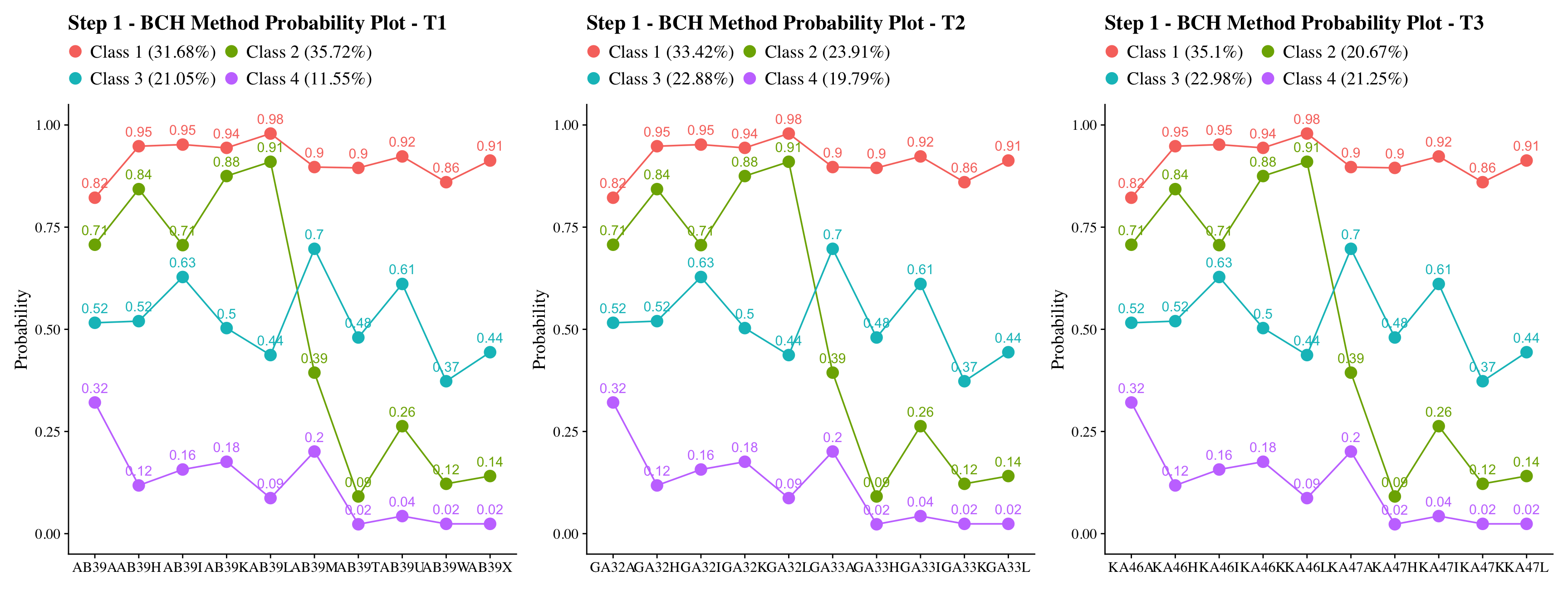
28.19.2 BCH Step 2: Extract BCH weights
bch_savedata <- as.data.frame(inv_bch$savedata)
#summary(bch_savedata)
28.19.3 BCH Step 3a: Estimate the Unconditional LTA Model Using BCH Weights
step3_bch  <- mplusObject(
  TITLE = "Step 3 - BCH Method",

  VARIABLE =
 "usevar = BCHW1-BCHW64;

  training = BCHW1-BCHW64(bch);

  classes = c1(4) c2(4) c3(4);" ,

  ANALYSIS =
 "type = mixture;
  starts = 0;",

  MODEL = glue(
  "%overall%

  c2 ON c1;
  c3 ON c2;"),

  usevariables = colnames(bch_savedata),
  rdata = bch_savedata)

step3_fit_bch <- mplusModeler(step3_bch,
               dataout=here("three_lta", "phase_3", "step_3a_bch", "step3.dat"),
               modelout=here("three_lta", "phase_3", "step_3a_bch", "unconditional_bch.inp"),
               check=TRUE, run = TRUE, hashfilename = FALSE)
28.19.3.1 Plotting BCH Transition Probabilities
source(here("functions","plot_transition.R"))

lta_model <- readModels(here("three_lta", "phase_3", "step_3a_bch", "unconditional_bch.out"))

plot_transition(
  model_name = lta_model,
  facet_labels = c(`1` = "Very Positive", `2` = "Qualified Positive", `3` = "Neutral", `4` = "Less Positive"),
  timepoint_labels = c(`1` = "Grade 7", `2` = "Grade 10", `3` = "Grade 12"),
  class_labels = c(`1` = "Very Positive", `2` = "Qualified Positive", `3` = "Neutral", `4` = "Less Positive")
) +
  labs(title = "Unconditional LTA (BCH Method)")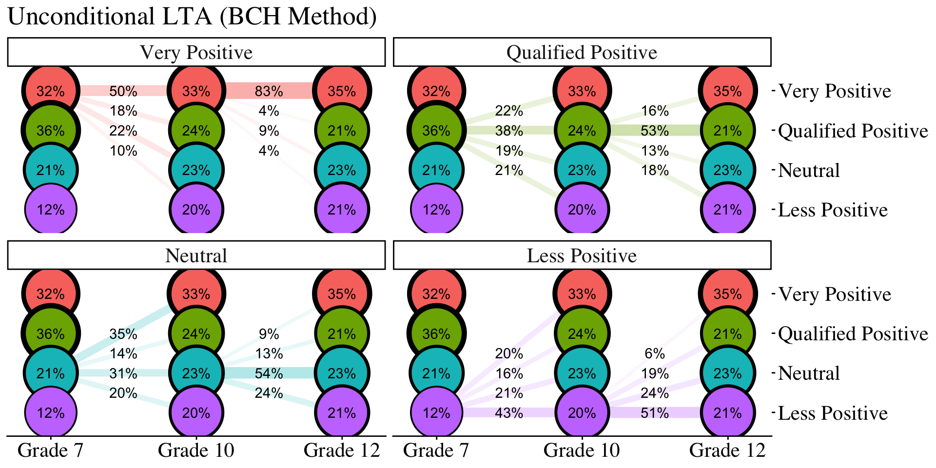
ggsave(here("figures", "unconditional_lta_bch.jpeg"), dpi="retina", height = 6, width = 10, bg = "white", units="in")28.19.4 BCH Step 3b: Estimate the Covariate-Adjusted LTA Model Using BCH Weights
step3_bch  <- mplusObject(
  TITLE = "Step 3 - BCH Method",

  VARIABLE =
 "usevar = BCHW1-BCHW64 MINORITY, FEMALE;

  training = BCHW1-BCHW64(bch);

  classes = c1(4) c2(4) c3(4);" ,

  ANALYSIS =
 "estimator = mlr;
  type = mixture;
  starts = 0;",

  MODEL =
  glue(
 " %OVERALL%

  c1 ON MINORITY Female;
  c2 ON c1 MINORITY Female;
  c3 ON c2 MINORITY Female;"),

  usevariables = colnames(bch_savedata),
  rdata = bch_savedata)

step3_fit_bch <- mplusModeler(step3_bch,
               dataout=here("three_lta", "phase_3", "step_3b_bch", "step3.dat"),
               modelout=here("three_lta", "phase_3", "step_3b_bch", "bch_covariates.inp"),
               check=TRUE, run = TRUE, hashfilename = FALSE)
28.19.4.1 Covariate Table: BCH Method
lta_cov_model <- readModels(here("three_lta", "phase_3", "step_3b_bch", "bch_covariates.out"))

# REFERENCE CLASS 4
cov <- as.data.frame(lta_cov_model[["parameters"]][["unstandardized"]]) %>%
  filter(param %in% c("MINORITY", "FEMALE")) %>%
  mutate(param = case_when(
            param == "FEMALE" ~ "Gender",
            param == "MINORITY" ~ "URM"),
    se = paste0("(", format(round(se,2), nsmall =2), ")")) %>%
  separate(paramHeader, into = c("Time", "Class"), sep = "#") %>%
  mutate(Class = case_when(
            Class == "1.ON" ~ "Very Positive",
            Class == "2.ON" ~ "Qualified Positive",
            Class == "3.ON" ~ "Neutral"),
         Time = case_when(
            Time == "C1" ~ "7th Grade (T1)",
            Time == "C2" ~ "10th Grade (T2)",
            Time == "C3" ~ "12th Grade (T3)",
         )
         ) %>%
  unite(estimate, est, se, sep = " ") %>%
  select(Time:pval, -est_se) %>%
  mutate(pval = ifelse(pval<0.001, paste0("<.001*"),
                       ifelse(pval<0.05, paste0(scales::number(pval, accuracy = .001), "*"),
                              scales::number(pval, accuracy = .001))))


# Create table

cov_m1 <- cov %>%
  group_by(param, Class) %>%
  gt() %>%
  tab_header(
    title = "Relations Between the Covariates and Latent Class (BCH Method)") %>%
  tab_footnote(
    footnote = md(
      "Reference Group: Less Positive"
    ),
locations = cells_title()
  ) %>%
  cols_label(
    param = md("Covariate"),
    estimate = md("Estimate (*se*)"),
    pval = md("*p*-value")) %>%
  sub_missing(1:3,
              missing_text = "") %>%
  sub_values(values = c(999.000), replacement = "-") %>%
  cols_align(align = "center") %>%
  opt_align_table_header(align = "left") %>%
  gt::tab_options(table.font.names = "serif")

cov_m1| Relations Between the Covariates and Latent Class (BCH Method)1 | ||
| Time | Estimate (se) | p-value |
|---|---|---|
| URM - Very Positive | ||
| 7th Grade (T1) | 0.225 (0.27) | 0.406 |
| 10th Grade (T2) | 0.442 (0.27) | 0.100 |
| 12th Grade (T3) | 0.809 (0.60) | 0.175 |
| Gender - Very Positive | ||
| 7th Grade (T1) | -0.655 (0.19) | 0.001* |
| 10th Grade (T2) | -0.091 (0.20) | 0.641 |
| 12th Grade (T3) | 0.338 (0.45) | 0.457 |
| URM - Qualified Positive | ||
| 7th Grade (T1) | 0.096 (0.28) | 0.736 |
| 10th Grade (T2) | 0.444 (0.27) | 0.105 |
| 12th Grade (T3) | 1.099 (0.40) | 0.006* |
| Gender - Qualified Positive | ||
| 7th Grade (T1) | 0.1 (0.20) | 0.621 |
| 10th Grade (T2) | 0.411 (0.20) | 0.039* |
| 12th Grade (T3) | 0.623 (0.27) | 0.022* |
| URM - Neutral | ||
| 7th Grade (T1) | 0.515 (0.32) | 0.103 |
| 10th Grade (T2) | 0.145 (0.31) | 0.640 |
| 12th Grade (T3) | 0.822 (0.40) | 0.039* |
| Gender - Neutral | ||
| 7th Grade (T1) | -0.431 (0.24) | 0.069 |
| 10th Grade (T2) | 0.062 (0.21) | 0.771 |
| 12th Grade (T3) | 0.372 (0.26) | 0.152 |
| 1 Reference Group: Less Positive | ||