9 Joint Occurrence

---

Example: Longitudinal Study of American Youth

Data source: : See documentation here

---

9.1 Load Packages

library(MplusAutomation)
library(tidyverse)
library(here)
library(glue)
library(gt)
library(cowplot)
library(kableExtra)
library(psych)
library(float)
library(janitor)
library(ggalluvial)
library(DiagrammeR)
library(modelsummary)
library(corrplot)
library(ggrepel)

---

9.2 Path Diagram

grViz("
digraph model {
    graph [layout=dot, overlap=true]

    node [shape=box]
    math_enjoy    [label=\"Math: Enjoy\"]    
    math_useful    [label=\"Math: Useful\"]
    math_logical   [label=\"Math: Logical\"]
    math_job       [label=\"Math: Job\"]
    math_adult     [label=\"Math: Adult\"]
    science_enjoy [label=\"Science: Enjoy\"]
    science_useful [label=\"Science: Useful\"]
    science_logical[label=\"Science: Logical\"]
    science_job    [label=\"Science: Job\"]
    science_adult  [label=\"Science: Adult\"]

    node [shape=circle]
    C_math [label=<C<SUB>Math</SUB>>];
    C_sci [label=<C<SUB>Science</SUB>>];

    edge []
    C_math -> {math_enjoy math_useful math_logical math_job math_adult}
    C_sci -> {science_enjoy science_useful science_logical science_job science_adult}
    C_math -> C_sci

    {rank = same; C_math; C_sci;}
}
")

---

LCA Indicators: Math and Science
Name	Description
Math
KA46A	I Enjoy Math
KA46H	Math is Useful in Everyday Problems
KA46I	Math Helps Logical Thinking
KA46K	Need Math for a Good Job
KA46L	Will Use Math Often as an Adult
Science
KA47A	I Enjoy Science
KA47H	Science is Useful in Everyday Problems
KA47I	Science Helps Logical Thinking
KA47K	Need Science for a Good Job
KA47L	Will Use Science Often as an Adult

---

Read in LSAY dataset

data <- read_csv(here("data", "lsay_joint_occurrence.csv")) %>% 
  rename(
    math_enjoy   = KA46A, # Renaming the variables
    math_useful  = KA46H,
    math_logical = KA46I,
    math_job     = KA46K,
    math_adult   = KA46L,
    sci_enjoy   = KA47A,
    sci_useful  = KA47H,
    sci_logical = KA47I,
    sci_job     = KA47K,
    sci_adult   = KA47L
  ) %>% 
  clean_names() %>% # Making variables lower-case
  mutate(across(
    .cols = math_enjoy:sci_adult, # Dichtomizing the variables
    .fns = ~ case_when(
      . %in% c(1, 2) ~ 1,
      . %in% c(3, 4, 5) ~ 0,
      TRUE ~ NA_real_
    )
  ))

---

9.3 Descriptive Statistics

9.3.1 Descriptive Statistics using R:

Quick view of all the relevant variables:

data %>%
  select(
    math_enjoy, math_useful, math_logical, math_job, math_adult,
    sci_enjoy, sci_useful, sci_logical, sci_job, sci_adult
  ) %>%
  psych::describe()

Proportion of indicators using R:

# Set up data to find proportions of binary indicators
ds <- data %>% 
  pivot_longer(c(math_enjoy:sci_adult), names_to = "Variable") 

# Create table of variables and counts
tab <- table(ds$Variable, ds$value)

# Find proportions and round to 3 decimal places
prop <- prop.table(tab, margin = 1) %>% 
  round(3)

# Combine everything to one table 
dframe <- data.frame(Variables=rownames(tab), Proportion=prop[,2], Count=tab[,2])
#remove row names
row.names(dframe) <- NULL

# Create table
gt(dframe) %>% 
tab_header(title = md("**LCA Indicator Proportions**"), subtitle = md("&nbsp;")) %>%
tab_options(column_labels.font.weight = "bold", row_group.font.weight = "bold") %>% 
tab_row_group(group = "Math", rows = 1:5) %>% 
tab_row_group(group = "Science", rows = 6:10) %>%
row_group_order(groups = c("Math","Science")) %>% 
tab_options(column_labels.font.weight = "bold", row_group.font.weight = "bold") 

LCA Indicator Proportions
Variables	Proportion	Count
Math
math_adult	0.634	2121
math_enjoy	0.547	1847
math_job	0.567	1891
math_logical	0.680	2279
math_useful	0.635	2131
Science
sci_adult	0.403	1352
sci_enjoy	0.534	1793
sci_job	0.341	1139
sci_logical	0.548	1825
sci_useful	0.450	1502

Data summary:

select_data <- data %>% 
 select(math_enjoy:sci_adult)

f <- All(select_data) ~ Mean + SD + Min + Median + Max + Histogram
datasummary(f, data, output="markdown")

	Mean	SD	Min	Median	Max	Histogram
math_enjoy	0.55	0.50	0.00	1.00	1.00	▆▇
math_useful	0.63	0.48	0.00	1.00	1.00	▄▇
math_logical	0.68	0.47	0.00	1.00	1.00	▃▇
math_job	0.57	0.50	0.00	1.00	1.00	▅▇
math_adult	0.63	0.48	0.00	1.00	1.00	▄▇
sci_enjoy	0.53	0.50	0.00	1.00	1.00	▆▇
sci_useful	0.45	0.50	0.00	0.00	1.00	▇▆
sci_logical	0.55	0.50	0.00	1.00	1.00	▆▇
sci_job	0.34	0.47	0.00	0.00	1.00	▇▄
sci_adult	0.40	0.49	0.00	0.00	1.00	▇▅

Correlation table:

select_data %>% 
  datasummary_correlation(output = "markdown")

	math_enjoy	math_useful	math_logical	math_job	math_adult	sci_enjoy	sci_useful	sci_logical	sci_job	sci_adult
math_enjoy	1	.	.	.	.	.	.	.	.	.
math_useful	.31	1	.	.	.	.	.	.	.	.
math_logical	.32	.51	1	.	.	.	.	.	.	.
math_job	.31	.43	.38	1	.	.	.	.	.	.
math_adult	.36	.55	.41	.53	1	.	.	.	.	.
sci_enjoy	.23	.23	.25	.22	.24	1	.	.	.	.
sci_useful	.21	.41	.36	.31	.33	.43	1	.	.	.
sci_logical	.21	.33	.48	.32	.30	.45	.58	1	.	.
sci_job	.22	.26	.27	.42	.29	.37	.50	.43	1	.
sci_adult	.22	.30	.28	.29	.37	.48	.54	.47	.62	1

Correlation plot:

f_cor <- data %>% 
 select(math_enjoy:sci_adult) %>% 
  cor(use = "pairwise.complete.obs")

corrplot(f_cor, 
         method = "circle",
         type = "upper", 
         tl.col="black", 
         tl.srt=45)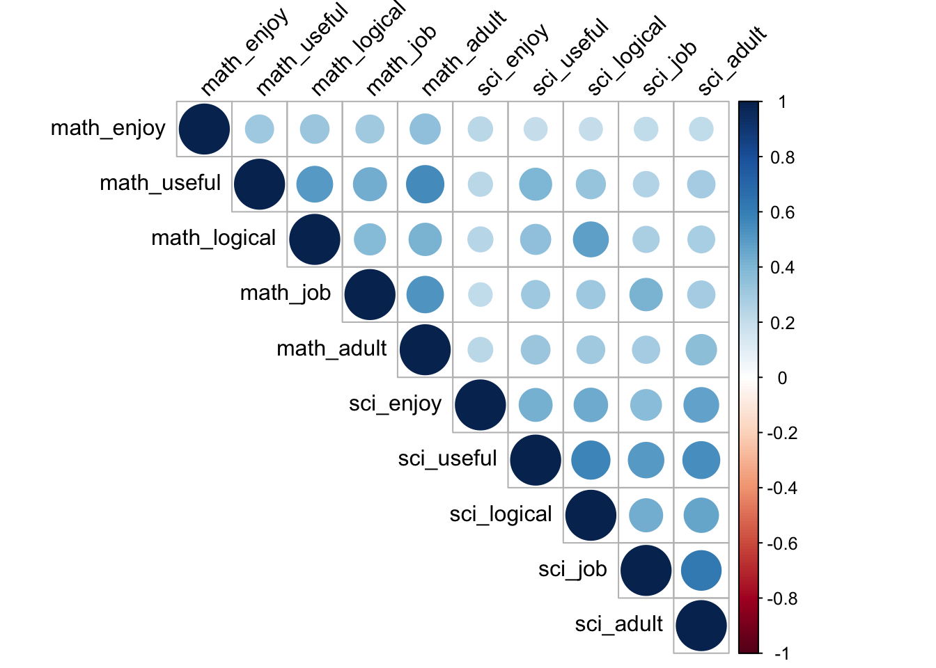

9.3.2 Descriptive Statistics using MplusAutomation:

basic_mplus  <- mplusObject(
  TITLE = "Descriptive Statistics;",
  
  VARIABLE =
    "usevar = math_enjoy-sci_adult;
    categorical = math_enjoy-sci_adult;",

  ANALYSIS = "TYPE=basic;",
  
  OUTPUT = "sampstat;",  
  
  usevariables = colnames(data),
  rdata = data)

basic_mplus_fit <- mplusModeler(basic_mplus, 
                            dataout = here("joint_occurrence", "data.dat"),
                            modelout = here("joint_occurrence","basic.inp"),
                            check = TRUE, run = TRUE, hashfilename = FALSE)

View output (which is goes more into detail) or a see a brief view of descriptive statistics using get_sampstat():

# Using MplusAutomation
MplusAutomation::get_sampstat(basic_mplus_fit)

# Using base R
summary(data)

---

9.4 Enumeration (Math Only)

This code uses the mplusObject function in the MplusAutomation package and saves all model runs in the mplus_enum folder.

lca_enum_6  <- lapply(1:6, function(k) {
  lca_enum  <- mplusObject(
    
    TITLE = glue("Math Attitudes: {k}-Class"), 
    
    VARIABLE = glue(
      "categorical = math_enjoy, math_useful, math_logical, math_job, math_adult; 
     usevar = math_enjoy, math_useful, math_logical, math_job, math_adult;
     classes = c({k});"),
    
    ANALYSIS = 
      "estimator = mlr; 
    type = mixture;
    processors = 12;
    starts = 500 100;",
    
    OUTPUT = "sampstat residual tech11 tech14;",

    usevariables = colnames(data),
    rdata = data)
  
  lca_enum_fit <- mplusModeler(lca_enum, 
                               dataout=glue(here("joint_occurrence","enum_math", "data.dat")),
                               modelout=glue(here("joint_occurrence","enum_math", "c{k}_math.inp")) ,
                               check=TRUE, run = TRUE, hashfilename = FALSE)
})

IMPORTANT: Before moving forward, make sure to examine each output document to ensure models were estimated normally. In this example, the last model (6-class models) did not produce reliable output and was excluded.

---

9.5 Enumeration (Science Only)

This code uses the mplusObject function in the MplusAutomation package and saves all model runs in the mplus_enum folder.

lca_enum_6  <- lapply(1:6, function(k) {
  lca_enum  <- mplusObject(
    
    TITLE = glue("Science Attitudes: {k}-Class"), 
    
    VARIABLE = glue(
      "categorical = sci_enjoy, sci_useful, sci_logical, sci_job, sci_adult; 
     usevar = sci_enjoy, sci_useful, sci_logical, sci_job, sci_adult;
     classes = c({k});"),
    
    ANALYSIS = 
      "estimator = mlr; 
    type = mixture;
    processors = 12;
    starts = 500 100;",
    
    OUTPUT = "sampstat residual tech11 tech14;",

    usevariables = colnames(data),
    rdata = data)
  
  lca_enum_fit <- mplusModeler(lca_enum, 
                               dataout=glue(here("joint_occurrence","enum_sci", "data.dat")),
                               modelout=glue(here("joint_occurrence","enum_sci", "c{k}_sci.inp")) ,
                               check=TRUE, run = TRUE, hashfilename = FALSE)
})

IMPORTANT: Before moving forward, make sure to examine each output document to ensure models were estimated normally. In this example, the last model (6-class models) did not produce reliable output and was excluded.

---

9.5.0.1 Fit Table

source(here("functions", "enum_table_jo.R"))

# Read model outputs
output_enum_c1 <- readModels(here("joint_occurrence", "enum_math"), quiet = TRUE)
output_enum_c2 <- readModels(here("joint_occurrence", "enum_sci"), quiet = TRUE)

# Define rows for row groups (assuming 6 models per time)
rows_m1 <- 1:6
rows_m2 <- 7:12

fit_table_jo <- fit_table_jo(output_enum_c1, output_enum_c2, rows_m1, rows_m2)
fit_table_jo

Model Fit Summary Table1
Classes	Par	LL	BIC	aBIC	CAIC	AWE	BLRT	VLMR	BF	cmP_k
LCA 1
Math Attitudes: 1-Class	5	−11,112.23	22,265.10	22,249.22	22,270.10	22,320.74	–	–	0.0	<.001
Math Attitudes: 2-Class	11	−9,368.02	18,825.46	18,790.50	18,836.45	18,947.86	<.001	<.001	0.0	<.001
Math Attitudes: 3-Class	17	−9,243.39	18,624.95	18,570.93	18,641.95	18,814.12	<.001	<.001	0.0	<.001
Math Attitudes: 4-Class	23	−9,204.49	18,595.93	18,522.84	18,618.93	18,851.86	<.001	0.10	>100	1.00
Math Attitudes: 5-Class	29	−9,197.51	18,630.72	18,538.57	18,659.72	18,953.42	0.04	0.00	>100	<.001
Math Attitudes: 6-Class	35	−9,197.04	18,678.55	18,567.34	18,713.55	19,068.02	1.00	0.48	–	<.001
LCA 2
Science Attitudes: 1-Class	5	−11,315.87	22,672.34	22,656.45	22,677.34	22,727.94	–	–	0.0	<.001
Science Attitudes: 2-Class	11	−9,009.08	18,107.48	18,072.53	18,118.48	18,229.81	<.001	<.001	0.0	<.001
Science Attitudes: 3-Class	17	−8,814.56	17,767.18	17,713.17	17,784.18	17,956.24	<.001	<.001	0.0	<.001
Science Attitudes: 4-Class	23	−8,742.24	17,671.26	17,598.17	17,694.26	17,927.04	<.001	<.001	>100	1.00
Science Attitudes: 5-Class	29	−8,734.82	17,705.15	17,613.01	17,734.15	18,027.66	<.001	0.01	>100	<.001
Science Attitudes: 6-Class	35	−8,732.97	17,750.16	17,638.95	17,785.17	18,139.40	1.00	0.48	–	<.001
1 Note. Par = Parameters; LL = model log likelihood; BIC = Bayesian information criterion; aBIC = sample size adjusted BIC; CAIC = consistent Akaike information criterion; AWE = approximate weight of evidence criterion; BLRT = bootstrapped likelihood ratio test p-value; VLMR = Vuong-Lo-Mendell-Rubin adjusted likelihood ratio test p-value; cmPk = approximate correct model probability.

---

Save table:

gtsave(fit_table_jo, here("figures", "fit_table_jo.png"))

---

9.5.1 Information Criteria Plot

source(here("functions", "ic_plot_lca.R"))
ic_plot(output_enum_c1)

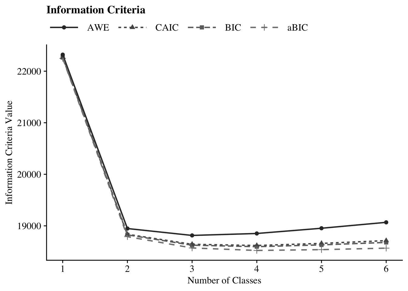
#ggsave(here("figures", "info_criteria_jo1.png"),  dpi = "retina", bg = "white", height=5, width=7, units="in")
ic_plot(output_enum_c2)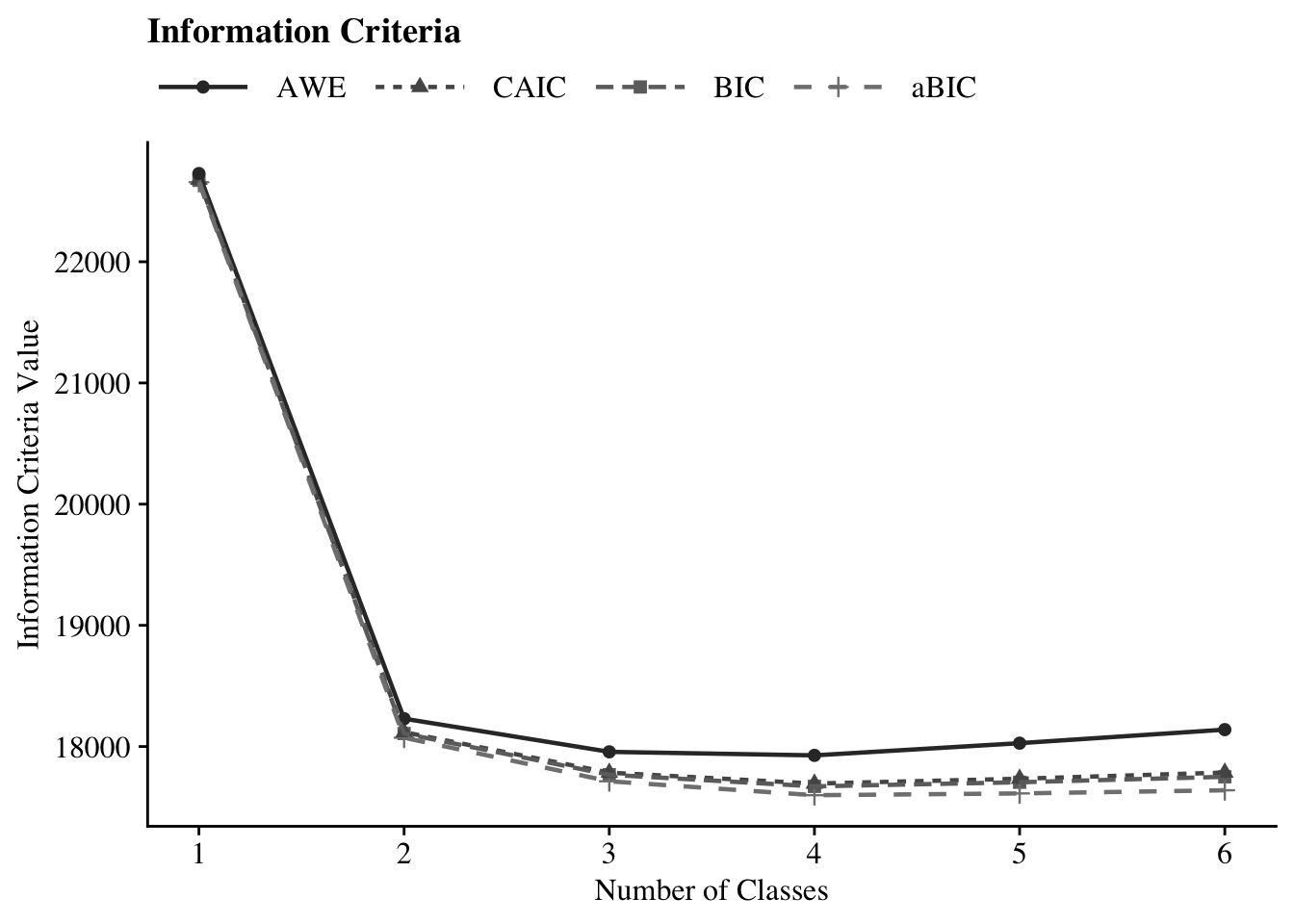

#ggsave(here("figures", "info_criteria_jo2.png"),  dpi = "retina", bg = "white", height=5, width=7, units="in")

---

9.5.2 4-Class Probability Plot

Use the plot_lca function provided in the folder to plot the item probability plot. This function requires one argument: - model_name: The name of the Mplus readModels object (e.g., output_enum_c1$c4_math.out)

source(here("functions","plot_lca.R"))

plot_lca(model_name = output_enum_c1$c4_math.out)

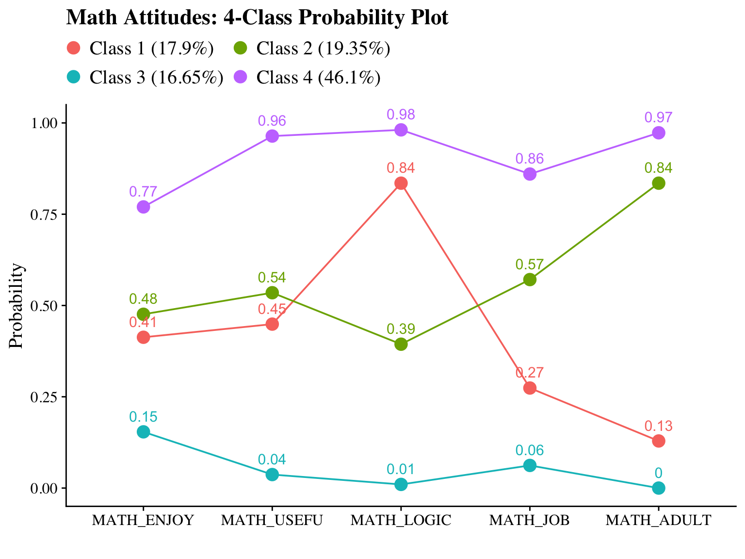
#ggsave(here("figures", "probability_plot_jo1.png"), dpi = "retina", bg = "white", height=5, width=7, units="in")
plot_lca(model_name = output_enum_c2$c4_sci.out)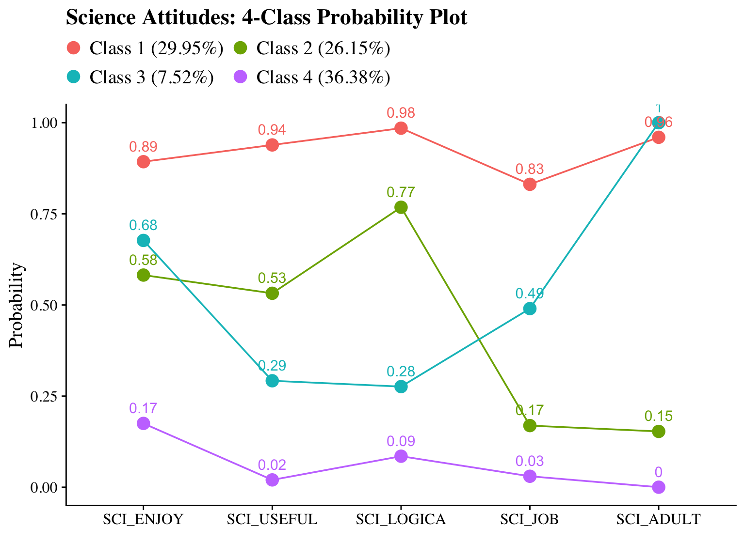

#ggsave(here("figures", "probability_plot_jo2.png"), dpi = "retina", bg = "white", height=5, width=7, units="in")

---

9.6 Estimate Joint Occurrence LCA

---

9.6.1 Step 1 - Estimate Unconditional Model

Math Attitudes

Here, I included the ID variable (casenum) so I can later join the two datasets we get from step 2.

step1  <- mplusObject(
  TITLE = "Step 1 - Unconditional Model", 
  VARIABLE = "categorical = math_enjoy, math_useful, math_logical, math_job, math_adult;
  usevar =  math_enjoy, math_useful, math_logical, math_job, math_adult;
  idvariable = casenum; 
  classes = c(4);",
  
  ANALYSIS = 
   "estimator = mlr; 
    type = mixture;
    starts = 0;
    OPTSEED = 830570;",
  
  SAVEDATA = 
   "File=savedata_math.dat;
    Save=cprob;",
  
  OUTPUT = "sampstat residual tech11 tech14 svalues(4 1 2 3)",  # I used `svalues` to rearrange the class labels
  
  usevariables = colnames(data),
  rdata = data)

step1_fit <- mplusModeler(step1,
                            dataout=here("joint_occurrence", "jo_model", "data.dat"),
                            modelout=here("joint_occurrence", "jo_model",  "one_math.inp") ,
                            check=TRUE, run = TRUE, hashfilename = FALSE)

Note: Since the emerging classes are similar between math and science, I rearranged the classes so that they match using svaues option in the OUTPUT command. For example, Class 1 of Science LCA and Class 4 of Math LCA are both the “High” class. So I changed the Math class from Class 4 to Class 1. Evaluate output and compare the class counts and proportions for the latent classes. Using the OPTSEED function ensures replication of the best loglikelihood value run.

---

Science Attitudes

step1  <- mplusObject(
  TITLE = "Step 1 - Unconditional Model", 
  VARIABLE = "categorical = sci_enjoy, sci_useful, sci_logical, sci_job, sci_adult;
  usevar =  sci_enjoy, sci_useful, sci_logical, sci_job, sci_adult;
  idvariable = casenum;
  classes = c(4);",
  
  ANALYSIS = 
   "estimator = mlr; 
    type = mixture;
    starts = 0;
    OPTSEED = 761633;",
  
  SAVEDATA = 
   "File=savedata_sci.dat;
    Save=cprob;",
  
  OUTPUT = "sampstat residual tech11 tech1;",
  
  usevariables = colnames(data),
  rdata = data)

step1_fit <- mplusModeler(step1,
                            dataout=here("joint_occurrence", "jo_model", "data.dat"),
                            modelout=here("joint_occurrence", "jo_model",  "one_sci.inp") ,
                            check=TRUE, run = TRUE, hashfilename = FALSE)

---

Confirm that plots look as expected (i.e., identical to enumeration model)

source(here("functions","plot_lca.R"))

output_math <- readModels(here("joint_occurrence","jo_model","one_math.out"))
output_sci <- readModels(here("joint_occurrence","jo_model","one_sci.out"))

plot_lca(model_name = output_math)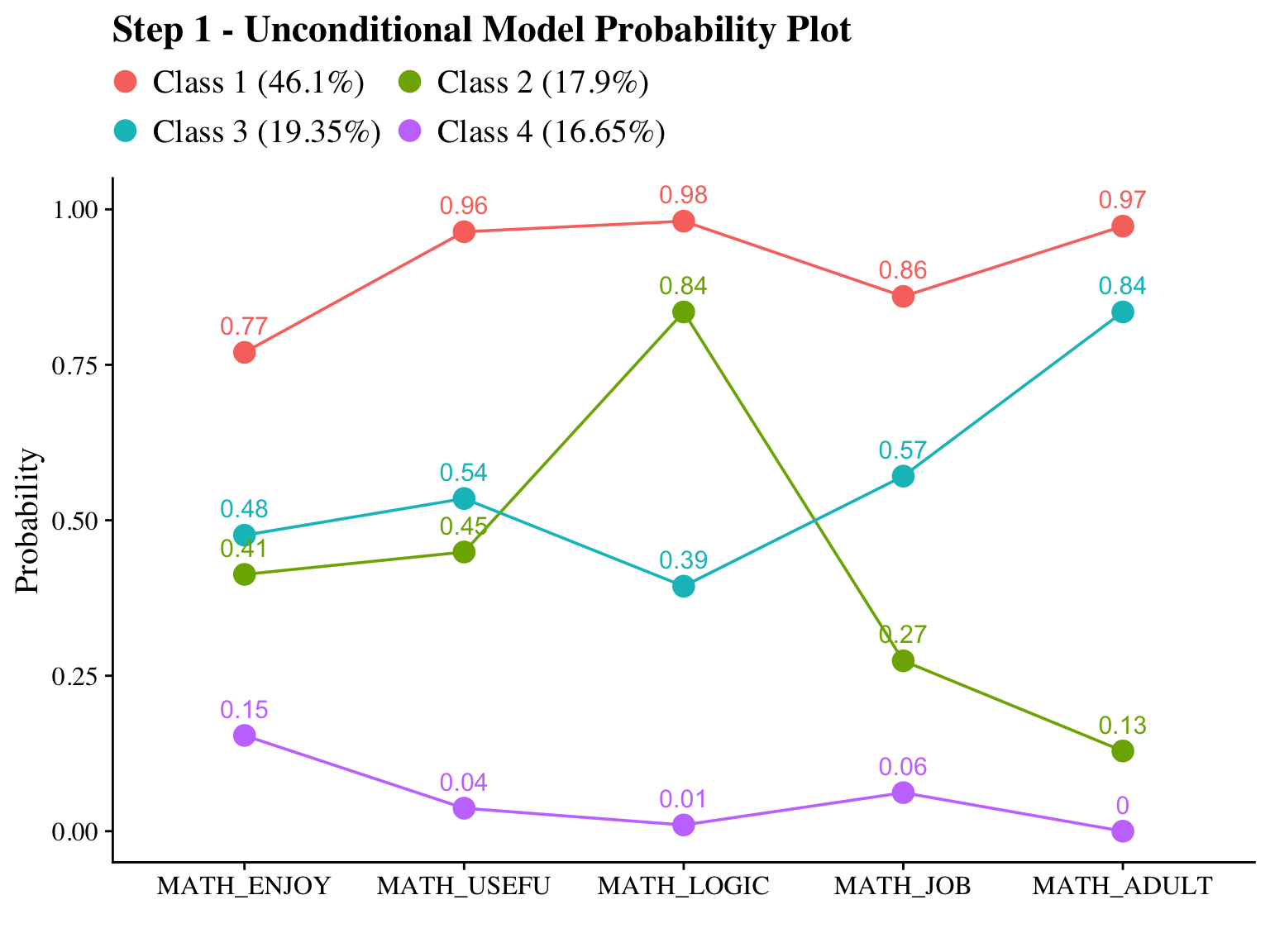

plot_lca(model_name = output_sci)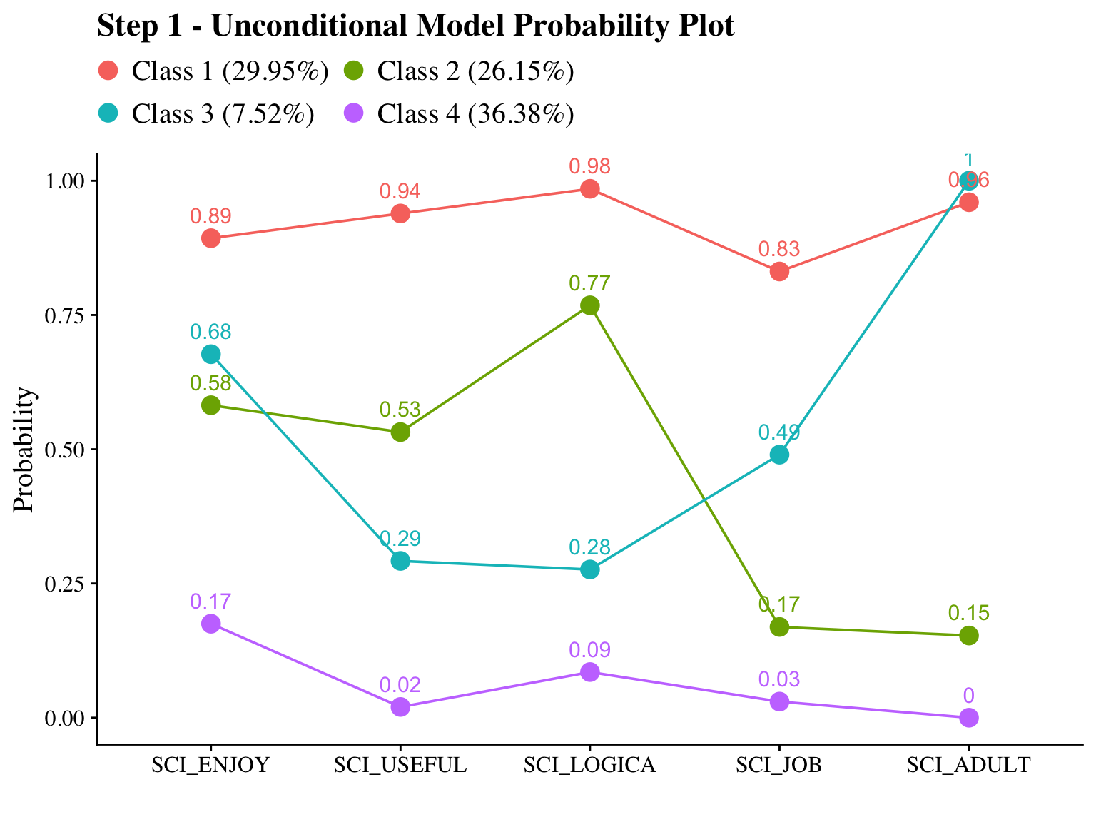

---

9.6.2 Step 2 - Determine Measurement Error

---

Extract logits for the classification probabilities for the most likely latent class:

logit_cprobs_math <- as.data.frame(output_math[["class_counts"]]
                                       [["logitProbs.mostLikely"]])

logit_cprobs_sci <- as.data.frame(output_sci[["class_counts"]]
                                       [["logitProbs.mostLikely"]])

Extract saved dataset:

savedata_math <- as.data.frame(output_math[["savedata"]])
savedata_sci <- as.data.frame(output_sci[["savedata"]])

Rename the column in savedata named “C” and change to “N”

colnames(savedata_math)[colnames(savedata_math)=="C"] <- "N_math"
colnames(savedata_sci)[colnames(savedata_sci)=="C"] <- "N_sci"

savedata <- savedata_math %>% 
  full_join(savedata_sci, by = "CASENUM")

---

9.6.3 Step 3 - Add Auxiliary Variables

---

Build the joint occurrence model:

step3_jo  <- mplusObject(
  TITLE = "Joint Occurrence LCA", 
  
  VARIABLE = 
 "nominal=N_math N_sci;
  usevar = N_math N_sci;
  classes = math(4) sci(4);" ,
  
  ANALYSIS = 
 "estimator = mlr; 
  type = mixture; 
  starts = 0;",
 
  MODEL =
  glue(
 " %OVERALL%
      
   sci on math; 

  MODEL math:
  
  %math#1%
  [N_math#1@{logit_cprobs_math[1,1]}];
  [N_math#2@{logit_cprobs_math[1,2]}];
  [N_math#3@{logit_cprobs_math[1,3]}];


  %math#2%
  [N_math#1@{logit_cprobs_math[2,1]}];
  [N_math#2@{logit_cprobs_math[2,2]}];
  [N_math#3@{logit_cprobs_math[2,3]}];
  
  %math#3%
  [N_math#1@{logit_cprobs_math[3,1]}]; 
  [N_math#2@{logit_cprobs_math[3,2]}];
  [N_math#3@{logit_cprobs_math[3,3]}];
  
  %math#4%
  [N_math#1@{logit_cprobs_math[4,1]}]; 
  [N_math#2@{logit_cprobs_math[4,2]}];
  [N_math#3@{logit_cprobs_math[4,3]}];  

 
  MODEL sci:
  
  %sci#1%
  [N_sci#1@{logit_cprobs_sci[1,1]}]; 
  [N_sci#2@{logit_cprobs_sci[1,2]}];
  [N_sci#3@{logit_cprobs_sci[1,3]}];  

  %sci#2%
  [N_sci#1@{logit_cprobs_sci[2,1]}];
  [N_sci#2@{logit_cprobs_sci[2,2]}];
  [N_sci#3@{logit_cprobs_sci[2,3]}];
  
  %sci#3%
  [N_sci#1@{logit_cprobs_sci[3,1]}];
  [N_sci#2@{logit_cprobs_sci[3,2]}];
  [N_sci#3@{logit_cprobs_sci[3,3]}];
 
  %sci#4%
  [N_sci#1@{logit_cprobs_sci[4,1]}];
  [N_sci#2@{logit_cprobs_sci[4,2]}];
  [N_sci#3@{logit_cprobs_sci[4,3]}];"),
 
  usevariables = colnames(savedata), 
  rdata = savedata)

step3_jo_fit <- mplusModeler(step3_jo,
               dataout=here("joint_occurrence","jo_model","three.dat"), 
               modelout=here("joint_occurrence","jo_model","three.inp"), 
               check=TRUE, run = TRUE, hashfilename = FALSE)

---

9.6.3.1 Joint Distribution

Plot:

jo_output <- readModels(here("joint_occurrence","jo_model","three.out"))

plot_lca(model_name = output_math)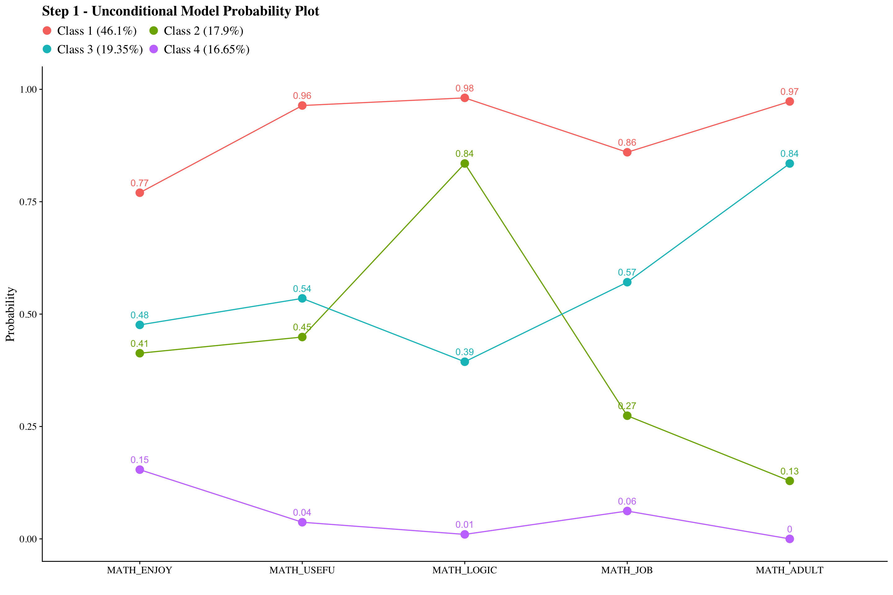

plot_lca(model_name = output_sci)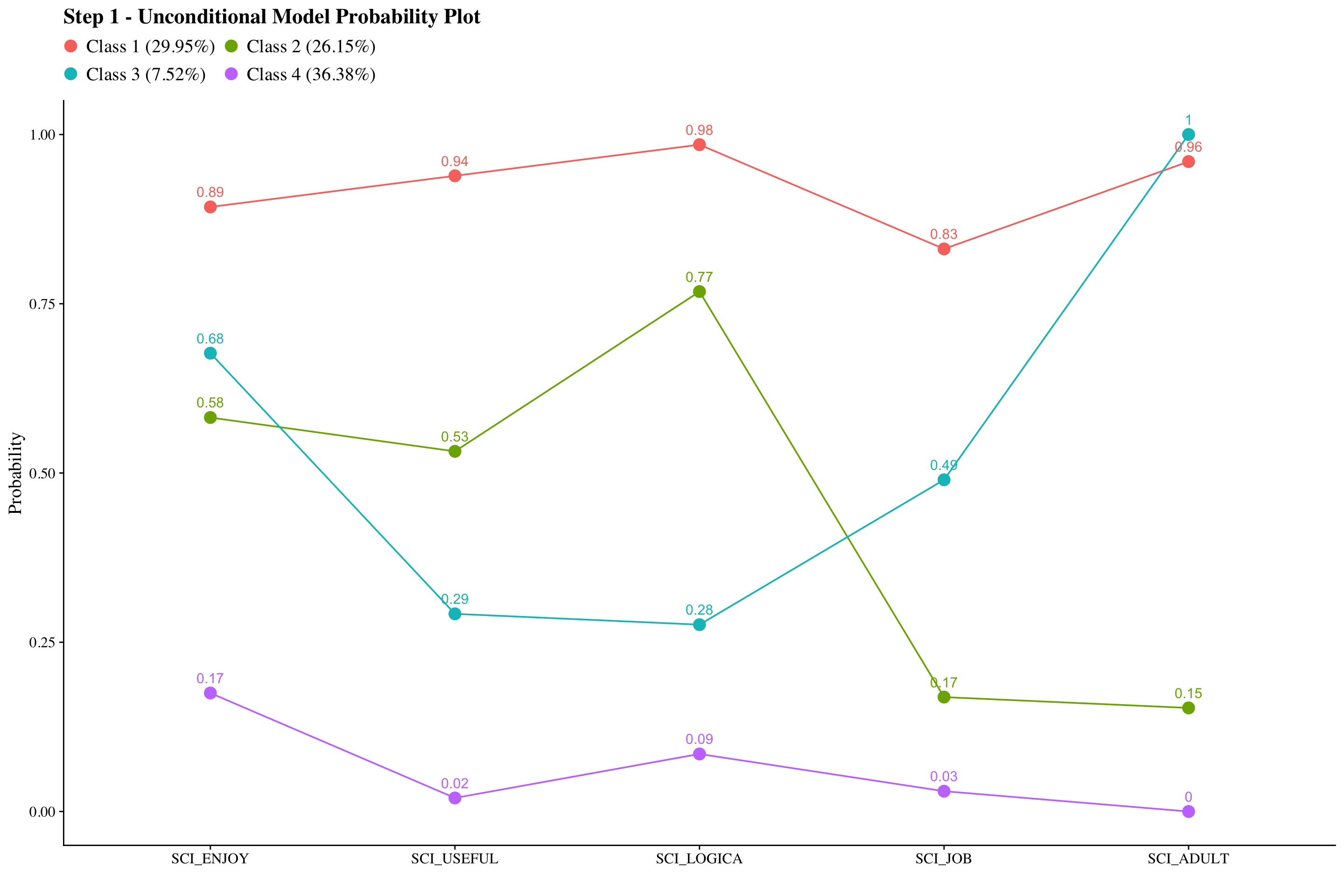

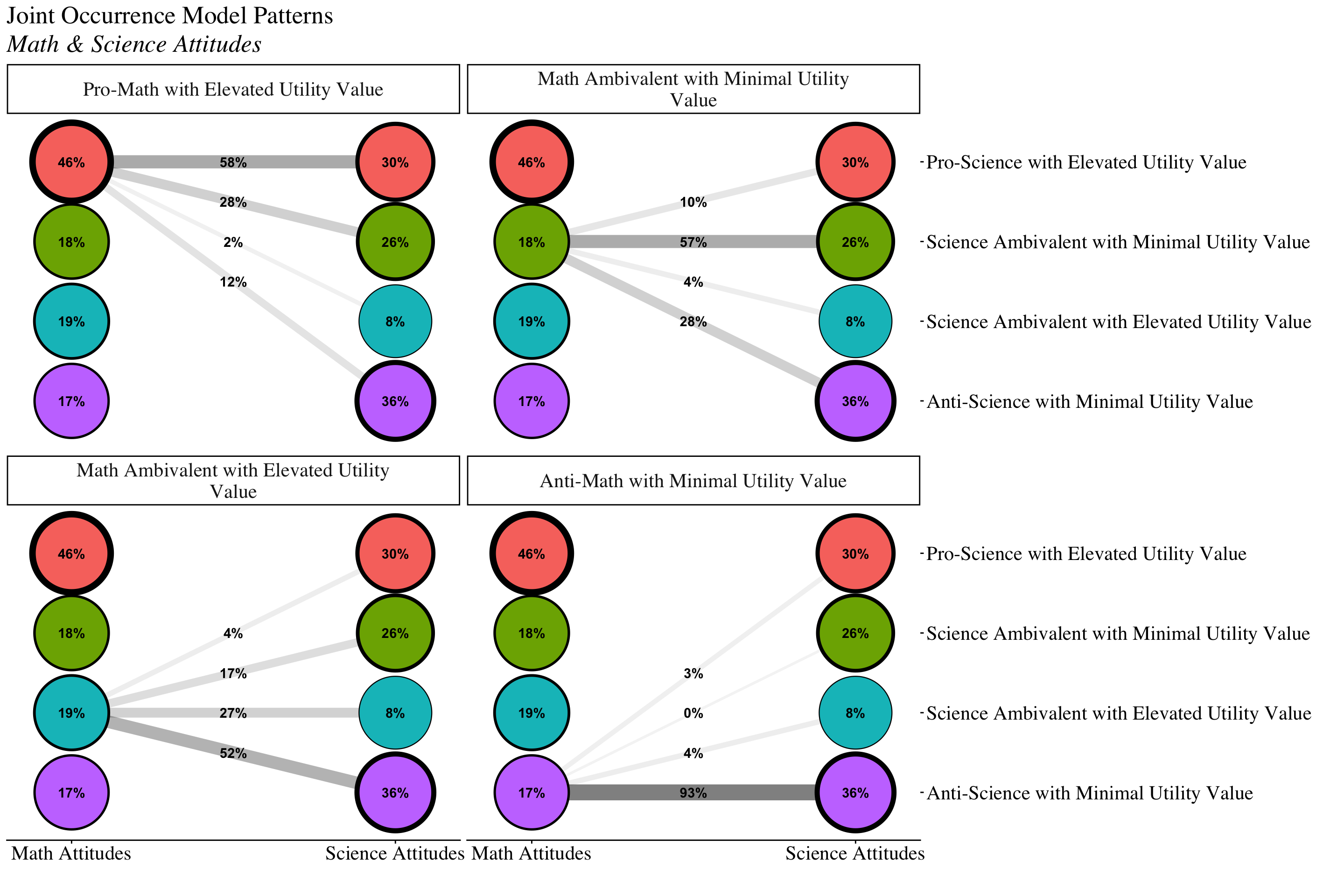
source(here("functions", "plot_patterns.R"))

title <- "Joint Occurrence Model Patterns"
subtitle <- "Math & Science Attitudes"

plot_patterns(
  model_name = jo_output,
  facet_labels =c(              # These are the Math labels
    `1` = "Pro-Math with Elevated Utility Value",
    `2` = "Math Ambivalent with Minimal Utility Value",
    `3` = "Math Ambivalent with Elevated Utility Value",
    `4` = "Anti-Math with Minimal Utility Value"),
  lca_labels = c('1' = "Math Attitudes", '2' = "Science Attitudes"), 
  class_labels = c(             # These are the Science labels
    "Pro-Science with Elevated Utility Value",
    "Science Ambivalent with Minimal Utility Value",
    "Science Ambivalent with Elevated Utility Value",
    "Anti-Science with Minimal Utility Value"
    ), 
  title,
  subtitle
  )

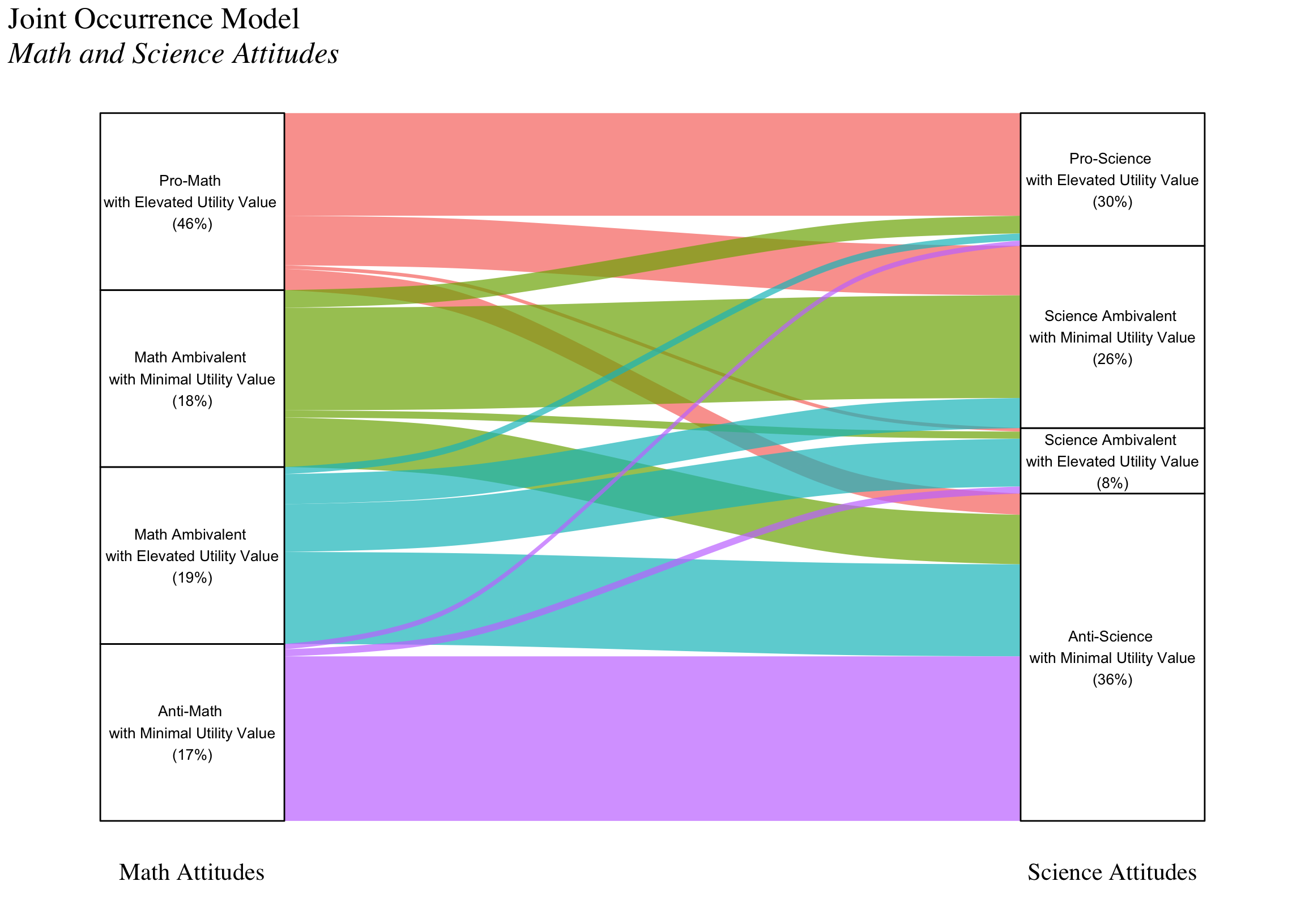
#ggsave(here("figures","interdependencies_plot.png"), dpi=500,bg = "white", height=7, width=12, units="in")

Alternative plot:

jo_output <- readModels(here("joint_occurrence","jo_model","three.out"))
jo_prob <- as.data.frame(jo_output$class_counts$transitionProbs$probability)

c1_labels <- c("Pro-Math \nwith Elevated Utility Value \n(46%)", 
               "Math Ambivalent \nwith Minimal Utility Value\n(18%)", 
               "Math Ambivalent \nwith Elevated Utility Value\n(19%)",
               "Anti-Math \nwith Minimal Utility Value\n(17%)")
c2_labels <- c("Pro-Science \nwith Elevated Utility Value\n(30%)",
               "Science Ambivalent \nwith Minimal Utility Value\n(26%)",
               "Science Ambivalent \nwith Elevated Utility Value\n(8%)",
               "Anti-Science \nwith Minimal Utility Value\n(36%)")


# T1 → T2
c1_c2 <- expand.grid(C1 = c1_labels, C2 = c2_labels) %>%
  mutate(P12 = jo_prob[1:nrow(jo_prob), 1]) %>% 
  mutate(P12 = round(P12, 2))


# Plot for T1 -> T2
 ggplot(c1_c2, aes(axis1 = C1, axis2 = C2, y = P12)) +
  geom_alluvium(aes(fill = C1), width = 0.2, alpha = 0.7) +
  # Make the stratum rectangles white instead of gray:
  geom_stratum(width = 0.2, color = "black") +
  geom_text(
    stat = "stratum", 
    aes(label = after_stat(stratum)), 
    size = 3.5
  ) +
  # Label the flows themselves with the probability
 # geom_text(aes(label = P12),
#            stat = "flow", nudge_x = .2, size = 5) +
  scale_x_discrete(limits = c("Math Attitudes", "Science Attitudes"), expand = c(.1, .1)) +
  labs(subtitle = "Math and Science Attitudes", title = "Joint Occurrence Model", x = "") +
  theme_minimal() +
  theme(
    text = element_text(family = "serif", size = 20),
    legend.position = "none",
    axis.text.x = element_text(color = "black"),
    axis.title.y = element_blank(),  
    axis.text.y  = element_blank(), 
    axis.ticks.y = element_blank(),
    panel.grid.major = element_blank(), 
    panel.grid.minor = element_blank(),  
    plot.subtitle = element_text(face = "italic", size = 20),
    plot.title = element_text(size = 20)
    )

#ggsave(here("figures", "jo_sankey.jpg"), width=8, height = 5.5, dpi="retina", bg = "white",  units="in")

Table:

# Extract Probabilities
jo_prob_matrix <- as.matrix(jo_output$class_counts$transitionProbs$probability)


# Label Classes
c1_labels <- c("Pro-Math \nwith Elevated Utility Value \n(46%)", 
               "Math Ambivalent \nwith Minimal Utility Value\n(18%)", 
               "Math Ambivalent \nwith Elevated Utility Value\n(19%)",
               "Anti-Math \nwith Minimal Utility Value\n(17%)")
c2_labels <- c("Pro-Science \nwith Elevated Utility Value\n(30%)",
               "Science Ambivalent \nwith Minimal Utility Value\n(26%)",
               "Science Ambivalent \nwith Elevated Utility Value\n(8%)",
               "Anti-Science \nwith Minimal Utility Value\n(36%)")

# Number of Classes for each LCA
C1 <- length(c1_labels)  
C2 <- length(c2_labels)  

# Format Probability Table
jo_df <- matrix(jo_prob_matrix, nrow = C1, ncol = C2, byrow = FALSE)
rownames(jo_df) <- c1_labels
colnames(jo_df) <- c2_labels
t_matrix <- as.data.frame(jo_df) %>%
  rownames_to_column(var = "Math Attitudes")

# Create Probability Table
t_matrix %>% 
  gt(rowname_col = "Math Attitudes") %>%
  tab_stubhead(label = "Math Attitudes") %>% 
  tab_header(
    title = md("**Joint Distribution Matrix**"),
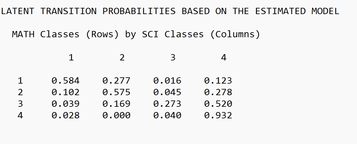
    subtitle = md("**Distribution Math Attitude Classes (Rows) conditioned on Science Attitude Classes (Columns)**")) %>% 
  fmt_number(2:4,decimals = 3) %>% 
  tab_spanner(label = "Science Attitudes",columns = 2:(C2+1))#%>% 

Joint Distribution Matrix
Distribution Math Attitude Classes (Rows) conditioned on Science Attitude Classes (Columns)
Math Attitudes	Science Attitudes
	Pro-Science with Elevated Utility Value (30%)	Science Ambivalent with Minimal Utility Value (26%)	Science Ambivalent with Elevated Utility Value (8%)	Anti-Science with Minimal Utility Value (36%)
Pro-Math with Elevated Utility Value (46%)	0.584	0.277	0.016	0.123
Math Ambivalent with Minimal Utility Value (18%)	0.102	0.575	0.045	0.278
Math Ambivalent with Elevated Utility Value (19%)	0.039	0.169	0.273	0.520
Anti-Math with Minimal Utility Value (17%)	0.028	0.000	0.040	0.932

  #gtsave("matrix.docx")

Always check the output to make sure the table is correct!