5 Including Auxiliary Variables
Example: PISA Student Data
Data source:
The first example utilizes a dataset on undergraduate Cheating available from the
poLCApackage (Dayton, 1998): See documentation hereThe second examples utilizes the public-use dataset, The Longitudinal Survey of American Youth (LSAY): See documentation here
5.1 Load packages
library(MplusAutomation)
library(tidyverse) #collection of R packages designed for data science
library(here) #helps with filepaths
library(janitor) #clean_names
library(gt) # create tables
library(cowplot) # a ggplot theme
library(DiagrammeR) # create path diagrams
library(glue) # allows us to paste expressions into R code
library(data.table) # used for `melt()` function
library(poLCA)
library(reshape2)
5.2 Automated Three-Step
Note: Prior to adding covariates or distals enumeration must be conducted. See Lab 6 for examples of enumeration with MplusAutomation.
Application: Undergraduate Cheating behavior
“Dichotomous self-report responses by 319 undergraduates to four questions about cheating behavior” (poLCA, 2016).
Prepare data
data(cheating)

cheating <- cheating %>% clean_names()

df_cheat <-  cheating %>%
  dplyr::select(1:4) %>%
  mutate_all(funs(.-1)) %>%
  mutate(gpa = cheating$gpa)

# Detaching packages that mask the dpylr functions
detach(package:poLCA, unload = TRUE)
detach(package:MASS, unload = TRUE)
5.2.1 DU3STEP in Mplus
DU3STEP incorporates distal outcome variables (assumed to have unequal means and variances) with mixture models.
5.2.1.1 Run the DU3step model with gpa as distal outcome
m_stepdu  <- mplusObject(
  TITLE = "DU3STEP - GPA as Distal",
  VARIABLE =
   "categorical = lieexam-copyexam;
    usevar = lieexam-copyexam;
    auxiliary = gpa (du3step);
    classes = c(2);",

  ANALYSIS =
   "estimator = mlr;
    type = mixture;
    starts = 500 100;
    processors = 10;",

  OUTPUT = "sampstat patterns tech11 tech14;",

  PLOT =
    "type = plot3;
     series = lieexam-copyexam(*);",

  usevariables = colnames(df_cheat),
  rdata = df_cheat)

m_stepdu_fit <- mplusModeler(m_stepdu,
                            dataout=here("three_step", "auto_3step", "du3step.dat"),
                            modelout=here("three_step", "auto_3step", "c2_du3step.inp") ,
                            check=TRUE, run = TRUE, hashfilename = FALSE)
5.2.1.2 Plot Distal Outcome mean differences
modelParams <- readModels(here("three_step", "auto_3step", "c2_du3step.out"))

# Extract class size
c_size <- as.data.frame(modelParams[["class_counts"]][["modelEstimated"]][["proportion"]]) %>%
  rename("cs" = 1) %>%
  mutate(cs = round(cs*100, 2))

c_size_val <- paste0("C", 1:nrow(c_size), glue(" ({c_size[1:nrow(c_size),]}%)"))


# Extract information as data frame
estimates <- as.data.frame(modelParams[["lcCondMeans"]][["overall"]]) %>%
  reshape2::melt(id.vars = "var") %>%
  mutate(variable = as.character(variable),
         LatentClass = case_when(
           endsWith(variable, "1") ~ c_size_val[1],
           endsWith(variable, "2") ~ c_size_val[2])) %>% #Add to this based on the number of classes you have
  head(-3) %>%
  pivot_wider(names_from = variable, values_from = value) %>%
  unite("mean", contains("m"), na.rm = TRUE) %>%
  unite("se", contains("se"), na.rm = TRUE) %>%
  mutate(across(c(mean, se), as.numeric))

# Add labels (NOTE: You must change the labels to match the significance testing!!)
value_labels <- paste0(estimates$mean, c(" a"," b"))

# Plot bar graphs
estimates %>%
  ggplot(aes(fill = LatentClass, y = mean, x = LatentClass)) +
  geom_bar(position = "dodge", stat = "identity", color = "black") +
  geom_errorbar(aes(ymin=mean-se, ymax=mean+se),
                size=.3,
                width=.2,
                position=position_dodge(.9)) +
  geom_text(aes(y = mean, label = value_labels),
            family = "serif", size = 4,
            position=position_dodge(.9),
            vjust = 8) +
  #scale_fill_grey(start = .5, end = .7) +
  labs(y="GPA", x="") +
  theme_cowplot() +
  theme(text = element_text(family = "serif", size = 12),
        axis.text.x = element_text(size=12),
        legend.position="none") +
  coord_cartesian(expand = FALSE,
                  ylim=c(0,max(estimates$mean*1.5))) # Change ylim based on distal outcome rang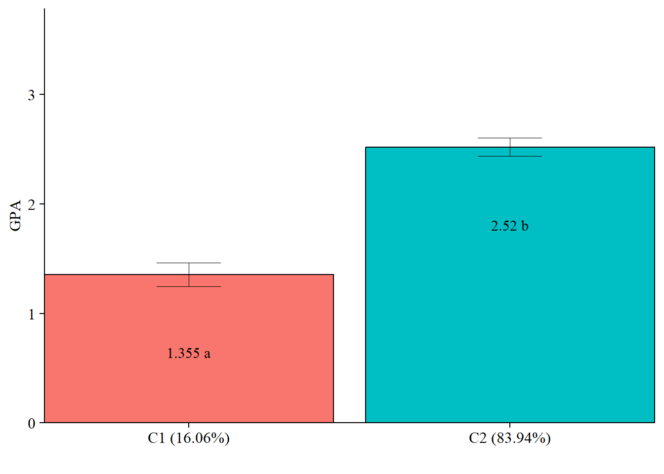
5.2.2 R3STEP
R3STEP incorporates latent class predictors with mixture models.
5.2.2.1 Run the R3STEP model with gpa as the latent class predictor
m_stepr  <- mplusObject(
  TITLE = "R3STEP - GPA as Predictor",
  VARIABLE =
   "categorical = lieexam-copyexam;
    usevar = lieexam-copyexam;
    auxiliary = gpa (R3STEP);
    classes = c(2);",

  ANALYSIS =
   "estimator = mlr;
    type = mixture;
    starts = 500 100;
    processors = 10;",

  OUTPUT = "sampstat patterns tech11 tech14;",

  PLOT =
    "type = plot3;
     series = lieexam-copyexam(*);",

  usevariables = colnames(df_cheat),
  rdata = df_cheat)

m_stepr_fit <- mplusModeler(m_stepr,
                            dataout=here("three_step", "auto_3step", "r3step.dat"),
                            modelout=here("three_step", "auto_3step", "c2_r3step.inp") ,
                            check=TRUE, run = TRUE, hashfilename = FALSE)
5.2.2.2 Regression slopes and odds ratios
TESTS OF CATEGORICAL LATENT VARIABLE MULTINOMIAL LOGISTIC REGRESSIONS USING
THE 3-STEP PROCEDURE

   WARNING:  LISTWISE DELETION IS APPLIED TO THE AUXILIARY VARIABLES IN THE
   ANALYSIS.  TO AVOID LISTWISE DELETION, DATA IMPUTATION CAN BE USED
   FOR THE AUXILIARY VARIABLES FOLLOWED BY ANALYSIS WITH TYPE=IMPUTATION.
   NUMBER OF DELETED OBSERVATIONS:  4
   NUMBER OF OBSERVATIONS USED:  315

                                                    Two-Tailed
                    Estimate       S.E.  Est./S.E.    P-Value

 C#1        ON
    GPA               -0.698      0.255     -2.739      0.006

 Intercepts
    C#1               -0.241      0.460     -0.523      0.601

Parameterization using Reference Class 1

 C#2        ON
    GPA                0.698      0.255      2.739      0.006

 Intercepts
    C#2                0.241      0.460      0.523      0.601


ODDS RATIOS FOR TESTS OF CATEGORICAL LATENT VARIABLE MULTINOMIAL LOGISTIC REGRESSIONS
USING THE 3-STEP PROCEDURE

                                                95% C.I.
                    Estimate       S.E. Lower 2.5% Upper 2.5%

 C#1        ON
    GPA                0.498      0.127      0.302      0.820


Parameterization using Reference Class 1

 C#2        ON
    GPA                2.009      0.512      1.220      3.310
5.3 Manual ML Three-step
Unlike the automatic three-step, the manual ML three-step can relate the latent class variable to both distal outcomes and covarites.
Integrate covariates and distals with a mixture model
Application: Longitudinal Study of American Youth, Science Attitudes
| LCA Indicators & Auxiliary Variables: Math Attitudes Example | |
| Name | Variable Description |
|---|---|
| enjoy | I enjoy math. |
| useful | Math is useful in everyday problems. |
| logical | Math helps a person think logically. |
| job | It is important to know math to get a good job. |
| adult | I will use math in many ways as an adult. |
| Auxiliary Variables | |
| female | Self-reported student gender (0=Male, 1=Female). |
| math_irt | Standardized IRT math test score - 12th grade. |
The data can be found in the data folder and is called lsay_subset.csv.
lsay_data <- read_csv(here("three_step","data","lsay_subset.csv")) %>%
  clean_names() %>%   # make variable names lowercase
  mutate(female = recode(gender, `1` = 0, `2` = 1)) # relabel values from 1,2 to 0,1
5.3.1 ML 3-Step Method
5.3.1.1 Step 1 - Class Enumeration w/ Auxiliary Specification
This step is done after class enumeration (or after you have selected the best latent class model). In this example, the four class model was the best. Now, we re-estimate the four-class model using optseed for efficiency. The difference here is the SAVEDATA command, where I can save the posterior probabilities and the modal class assignment that will be used in steps two and three.
step1  <- mplusObject(
  TITLE = "Step 1 - Three-Step using LSAL",
  VARIABLE =
  "categorical = enjoy useful logical job adult;
   usevar = enjoy useful logical job adult;

   classes = c(4);

   auxiliary =   ! list all potential covariates and distals here
   female  mothed      ! covariate
   math_irt;      ! distal math test score in 12th grade ",

  ANALYSIS =
   "estimator = mlr;
    type = mixture;
    starts = 0;
    optseed = 568405;",

  SAVEDATA =
   "File=3step_savedata.dat;
    Save=cprob;",

  OUTPUT = "residual tech11 tech14",

  PLOT =
    "type = plot3;
    series = enjoy-adult(*);",

  usevariables = colnames(lsay_data),
  rdata = lsay_data)

step1_fit <- mplusModeler(step1,
                            dataout=here("three_step", "manual_3step", "Step1.dat"),
                            modelout=here("three_step", "manual_3step", "one.inp") ,
                            check=TRUE, run = TRUE, hashfilename = FALSE)
source(here("functions", "plot_lca.R"))
output_lsay <- readModels(here("three_step", "manual_3step","one.out"))

plot_lca(model_name = output_lsay)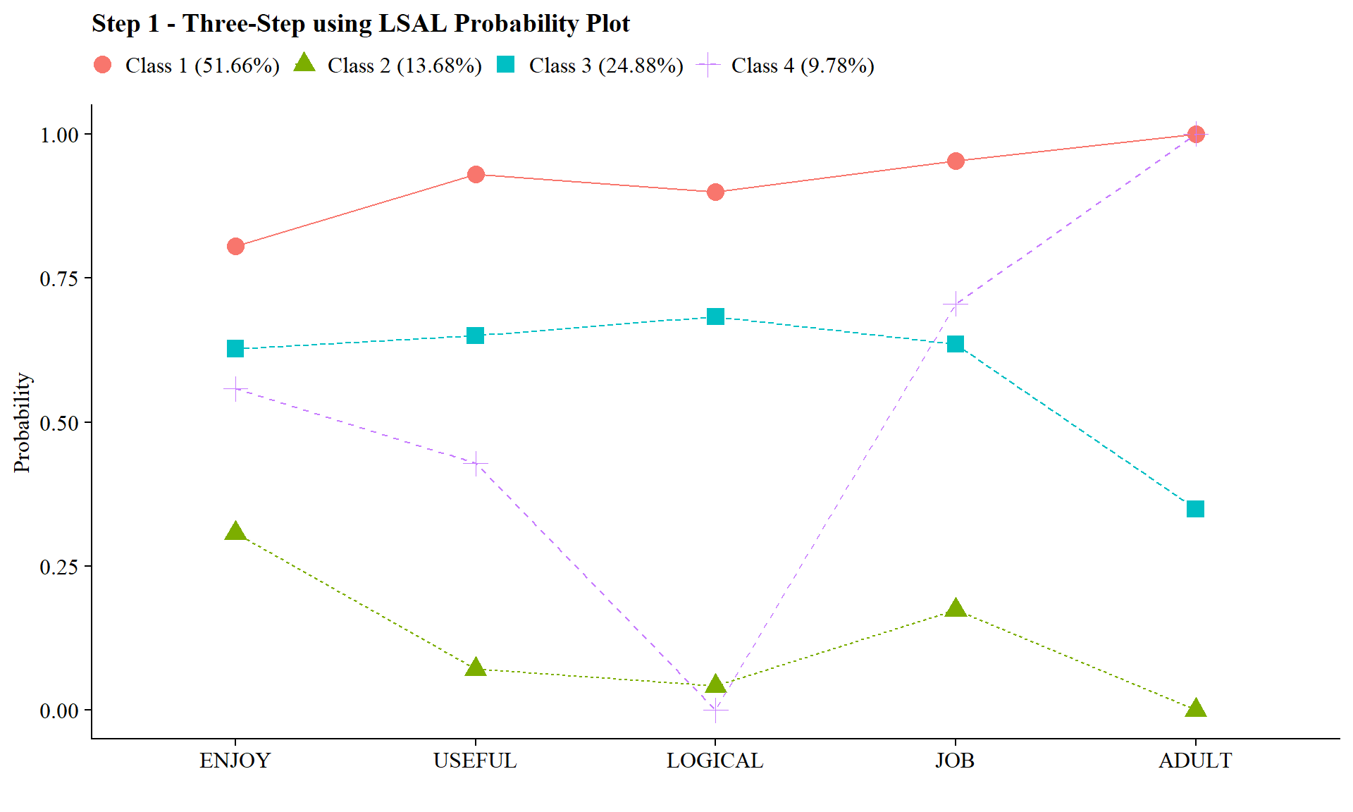
5.3.1.2 Step 2 - Determine Measurement Error
Extract logits for the classification probabilities for the most likely latent class
logit_cprobs <- as.data.frame(output_lsay[["class_counts"]]
                                       [["logitProbs.mostLikely"]])
Extract saved dataset which is part of the mplusObject “step1_fit”
savedata <- as.data.frame(output_lsay[["savedata"]])Rename the column in savedata named “C” and change to “N”
5.3.1.3 Step 3 - LCA Auxiliary Variable Model with 2 covariates and 1 distal outcome
5.3.1.3.1 Estimate LCA Model
Model with 2 covariates (gender and mother’s education) and 1 distal outcome (math IRT scores)
step3  <- mplusObject(
  TITLE = "Step3 - 3step LSAY",

  VARIABLE =
 "nominal=N;
  usevar = n;

  classes = c(4);

  usevar = female mothed math_irt;" ,

  ANALYSIS =
 "estimator = mlr;
  type = mixture;
  starts = 0;",

  DEFINE =
   "center female mothed (grandmean);",

  MODEL =
  glue(
 " %OVERALL%

  math_irt on female mothed; ! covariate as a related to the distal outcome
  C on female (f1-f3);
  c on mothed (e1-e3);      ! covariate as predictor of C

     %C#1%
  [n#1@{logit_cprobs[1,1]}]; ! MUST EDIT if you do not have a 4-class model.
  [n#2@{logit_cprobs[1,2]}];
  [n#3@{logit_cprobs[1,3]}];

  [math_irt](m1);    ! conditional distal mean
  math_irt;          ! conditional distal variance (freely estimated)

  %C#2%
  [n#1@{logit_cprobs[2,1]}];
  [n#2@{logit_cprobs[2,2]}];
  [n#3@{logit_cprobs[2,3]}];

  [math_irt](m2);
  math_irt;

  %C#3%
  [n#1@{logit_cprobs[3,1]}];
  [n#2@{logit_cprobs[3,2]}];
  [n#3@{logit_cprobs[3,3]}];

  [math_irt](m3);
  math_irt;

  %C#4%
  [n#1@{logit_cprobs[4,1]}];
  [n#2@{logit_cprobs[4,2]}];
  [n#3@{logit_cprobs[4,3]}];

  [math_irt](m4);
  math_irt; "),

  MODELCONSTRAINT =
   "New (diff12 diff13 diff23
    diff14 diff24 diff34

    d_fem_12 d_fem_13
    d_fem_23

    d_ed_12 d_ed_13
    d_ed_23
    );

    diff12 = m1-m2;  ! test pairwise distal mean differences
    diff13 = m1-m3;
    diff23 = m2-m3;
    diff14 = m1-m4;
    diff24 = m2-m4;
    diff34 = m3-m4;

    d_fem_12 = f1-f2;
    d_fem_13 = f1-f3;
    d_fem_23 = f2-f3;

    d_ed_12 = e1-e2;
    d_ed_13 = e1-e3;
    d_ed_23 = e2-e3;

 ",

  MODELTEST = "     ! omnibus test of distal means
  !  m1=m2;
  !  m2=m3;
  !  m3=m4;

  ! f1=f2;       ! omnibus test of covariate logits (female)
  !  f1=f3;

    e1=e2;       ! omnibus test of covariate logits (mothers ed)
    e1=e3;
   ",

  usevariables = colnames(savedata),
  rdata = savedata)

step3_fit <- mplusModeler(step3,
               dataout=here("three_step", "manual_3step", "Step3.dat"),
               modelout=here("three_step", "manual_3step", "three.inp"),
               check=TRUE, run = TRUE, hashfilename = FALSE)
5.3.1.3.2 Wald Test Table
This is testing if there is a relation between the latent class variable and the distal outcome (mathirt)
modelParams <- readModels(here("three_step", "manual_3step", "three.out"))

# Extract information as data frame
wald <- as.data.frame(modelParams[["summaries"]]) %>%
  dplyr::select(WaldChiSq_Value:WaldChiSq_PValue) %>%
  mutate(WaldChiSq_DF = paste0("(", WaldChiSq_DF, ")")) %>%
  unite(wald_test, WaldChiSq_Value, WaldChiSq_DF, sep = " ") %>%
  rename(pval = WaldChiSq_PValue) %>%
  mutate(pval = ifelse(pval<0.001, paste0("<.001*"),
                       ifelse(pval<0.05, paste0(scales::number(pval, accuracy = .001), "*"),
                              scales::number(pval, accuracy = .001))))

# Create table

wald_table <- wald %>%
  gt() %>%
    tab_header(
    title = "Wald Test Distal Means (Math IRT Scores)") %>%
    cols_label(
      wald_test = md("Wald Test (*df*)"),
      pval = md("*p*-value")) %>%
  cols_align(align = "center") %>%
  opt_align_table_header(align = "left") %>%
  gt::tab_options(table.font.names = "serif")

wald_table| Wald Test Distal Means (Math IRT Scores) | |
| Wald Test (df) | p-value |
|---|---|
| 69.134 (3) | <.001* |
Save figure
5.3.1.3.3 Table of Pairwise Distal Outcome Differences
modelParams <- readModels(here("three_step", "manual_3step", "three.out"))

# Extract information as data frame
diff <- as.data.frame(modelParams[["parameters"]][["unstandardized"]]) %>%
  filter(grepl("DIFF", param)) %>%
  dplyr::select(param:pval) %>%
  mutate(se = paste0("(", format(round(se,2), nsmall =2), ")")) %>%
  unite(estimate, est, se, sep = " ") %>%
  mutate(param = str_remove(param, "DIFF"),
         param = as.numeric(param)) %>%
  separate(param, into = paste0("Group", 1:2), sep = 1) %>%
  mutate(class = paste0("Class ", Group1, " vs ", Group2)) %>%
  dplyr::select(class, estimate, pval) %>%
  mutate(pval = ifelse(pval<0.001, paste0("<.001*"),
                       ifelse(pval<0.05, paste0(scales::number(pval, accuracy = .001), "*"),
                              scales::number(pval, accuracy = .001))))

# Create table

diff %>%
  gt() %>%
    tab_header(
    title = "Distal Outcome Differences") %>%
    cols_label(
      class = "Class",
      estimate = md("Mean (*se*)"),
      pval = md("*p*-value")) %>%
    sub_missing(1:3,
              missing_text = "") %>%
  cols_align(align = "center") %>%
  opt_align_table_header(align = "left") %>%
gt::tab_options(table.font.names = "serif")| Distal Outcome Differences | ||
| Class | Mean (se) | p-value |
|---|---|---|
| Class 1 vs 2 | 6.723 (0.98) | <.001* |
| Class 1 vs 3 | 3.108 (0.95) | 0.001* |
| Class 2 vs 3 | -3.615 (1.32) | 0.006* |
| Class 1 vs 4 | 7.034 (1.29) | <.001* |
| Class 2 vs 4 | 0.311 (1.45) | 0.830 |
| Class 3 vs 4 | 3.926 (1.49) | 0.008* |
5.3.1.3.4 Plot Distal Outcome Means
modelParams <- readModels(here("three_step", "manual_3step", "three.out"))

# Extract class size
c_size <- as.data.frame(modelParams[["class_counts"]][["modelEstimated"]][["proportion"]]) %>%
  rename("cs" = 1) %>%
  mutate(cs = round(cs*100, 2))

c_size_val <- paste0("C", 1:nrow(c_size), glue(" ({c_size[1:nrow(c_size),]}%)"))


# Extract information as data frame
estimates <- as.data.frame(modelParams[["parameters"]][["unstandardized"]]) %>%
  filter(paramHeader == "Intercepts") %>%
  dplyr::select(param, est, se) %>%
  filter(param == "MATH_IRT") %>%
  mutate(across(c(est, se), as.numeric)) %>%
  mutate(LatentClass = c_size_val)

# Add labels (NOTE: You must change the labels to match the significance testing!!)
#value_labels <- paste0(estimates$est, c("a"," bc"," abd"," cd"))

estimates$LatentClass <- fct_inorder(estimates$LatentClass)

# Plot bar graphs
estimates %>%
  ggplot(aes(x=LatentClass, y = est, fill = LatentClass)) +
  geom_col(position = "dodge", stat = "identity", color = "black") +
  geom_errorbar(aes(ymin=est-se, ymax=est+se),
                size=.3,    # Thinner lines
                width=.2,
                position=position_dodge(.9)) +
  geom_text(aes(label = est),
            family = "serif", size = 4,
            position=position_dodge(.9),
            vjust = 8) +
 # scale_fill_grey(start = .4, end = .7) + # Remove for colorful bars
  labs(y="Math Scores", x="") +
  theme_cowplot() +
  theme(text = element_text(family = "serif", size = 15),
        axis.text.x = element_text(size=15),
        legend.position="none")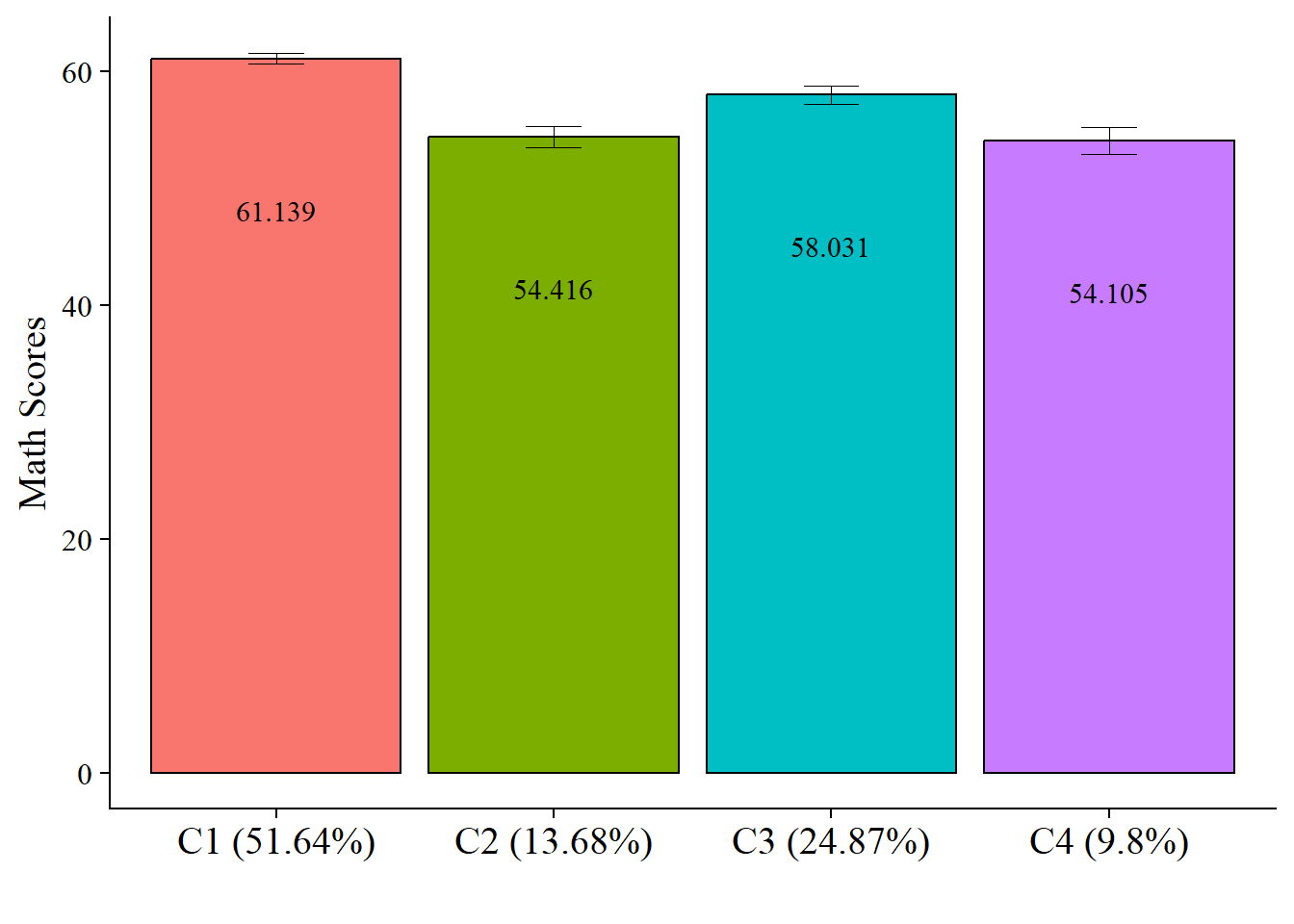
# Save plot
ggsave(here("figures","ManualDistal_Plot.jpeg"),
       dpi=300, width=10, height = 7, units="in")
5.3.1.3.5 Covariates Relations
modelParams <- readModels(here("three_step", "manual_3step", "three.out"))

# Extract information as data frame
cov <- as.data.frame(modelParams[["parameters"]][["unstandardized"]]) %>%
   filter(str_detect(paramHeader, "^C#\\d+\\.ON$")) %>%
  mutate(param = str_replace(param, "FEMALE", "Gender")) %>% # Change this to your own covariates
  mutate(param = str_replace(param, "MOTHED", "Mother's Education")) %>%
  mutate(est = format(round(est, 3), nsmall = 3),
         se = round(se, 2),
         pval = round(pval, 3)) %>%
  mutate(latent_class = str_replace(paramHeader, "^C#(\\d+)\\.ON$", "Class \\1")) %>%
  dplyr::select(param, est, se, pval, latent_class) %>%
  mutate(se = paste0("(", format(round(se,2), nsmall =2), ")")) %>%
  unite(logit, est, se, sep = " ") %>%
  dplyr::select(param, logit, pval, latent_class) %>%
  mutate(pval = ifelse(pval<0.001, paste0("<.001*"),
                       ifelse(pval<0.05, paste0(scales::number(pval, accuracy = .001), "*"),
                              scales::number(pval, accuracy = .001))))

or <- as.data.frame(modelParams[["parameters"]][["odds"]]) %>%
  filter(str_detect(paramHeader, "^C#\\d+\\.ON$")) %>%
  mutate(param = str_replace(param, "FEMALE", "Gender")) %>% # Change this to your own covariates
  mutate(param = str_replace(param, "MOTHED", "Mother's Education")) %>%
  mutate(est = format(round(est, 3), nsmall = 3)) %>%
  mutate(latent_class = str_replace(paramHeader, "^C#(\\d+)\\.ON$", "Class \\1")) %>%
  mutate(CI = paste0("[", format(round(lower_2.5ci, 3), nsmall = 3), ", ", format(round(upper_2.5ci, 3), nsmall = 3), "]")) %>%
  dplyr::select(param, est, CI, latent_class) %>%
  rename(or = est)

combined <- or %>%
  full_join(cov) %>%
  dplyr::select(param, latent_class, logit, pval, or, CI)


# Create table

combined %>%
  gt(groupname_col = "latent_class", rowname_col = "param") %>%
  tab_header(
    title = "Predictors of Class Membership") %>%
  cols_label(
    logit = md("Logit (*se*)"),
    or = md("Odds Ratio"),
    CI = md("95% CI"),
    pval = md("*p*-value")) %>%
  sub_missing(1:3,
              missing_text = "") %>%
  sub_values(values = c("999.000"), replacement = "-") %>%
  cols_align(align = "center") %>%
  opt_align_table_header(align = "left") %>%
  gt::tab_options(table.font.names = "serif") %>%
  tab_footnote(
    footnote = "Reference Class: 4",
    locations = cells_title(groups = "title")
)| Predictors of Class Membership1 | ||||
| Logit (se) | p-value | Odds Ratio | 95% CI | |
|---|---|---|---|---|
| Class 1 | ||||
| Gender | 0.166 (0.19) | 0.374 | 1.181 | [0.819, 1.704] |
| Class 2 | ||||
| Gender | 0.200 (0.20) | 0.330 | 1.221 | [0.817, 1.825] |
| Class 3 | ||||
| Gender | 0.107 (0.22) | 0.619 | 1.113 | [0.730, 1.699] |
| 1 Reference Class: 4 | ||||
5.3.1.3.6 Distal outcome regressed on the covariate
Is there a relation between the distal outcome (Math IRT Scores) and the covariate (Gender)?
modelParams <- readModels(here("three_step", "manual_3step", "three.out"))

# Extract information as data frame
donx <- as.data.frame(modelParams[["parameters"]][["unstandardized"]]) %>%
  filter(param %in% c("FEMALE", "MOTHED")) %>%
  mutate(param = str_replace(param, "FEMALE", "Gender")) %>%
  mutate(param = str_replace(param, "MOTHED", "Mother's Education")) %>%
  mutate(LatentClass = sub("^","Class ", LatentClass)) %>%
  dplyr::select(!paramHeader) %>%
  mutate(se = paste0("(", format(round(se,2), nsmall =2), ")")) %>%
    unite(estimate, est, se, sep = " ") %>%
  dplyr::select(param, estimate, pval) %>%
  distinct(param, .keep_all=TRUE) %>%
  mutate(pval = ifelse(pval<0.001, paste0("<.001*"),
                       ifelse(pval<0.05, paste0(scales::number(pval, accuracy = .001), "*"),
                              scales::number(pval, accuracy = .001))))


# Create table

donx %>%
  gt(groupname_col = "LatentClass", rowname_col = "param") %>%
  tab_header(
    title = "Gender Predicting Math Scores") %>%
  cols_label(
    estimate = md("Estimate (*se*)"),
    pval = md("*p*-value")) %>%
  sub_missing(1:3,
              missing_text = "") %>%
  sub_values(values = c("999.000"), replacement = "-") %>%
  cols_align(align = "center") %>%
  opt_align_table_header(align = "left") %>%
gt::tab_options(table.font.names = "serif")| Gender Predicting Math Scores | ||
| Estimate (se) | p-value | |
|---|---|---|
| Gender | -1.108 (0.55) | 0.045* |
5.3.1.4 Step 3 - LCA Auxiliary Variable Model with 1 covariate
5.3.1.4.1 Estimate LCA Model
step3  <- mplusObject(
  TITLE = "Step3 - 3step LSAY",

  VARIABLE =
 "nominal=N;
  usevar = n;

  classes = c(4);

  usevar = mothed math_irt;" ,

  ANALYSIS =
 "estimator = mlr;
  type = mixture;
  starts = 0;",

  DEFINE =
   "center mothed (grandmean);",

  MODEL =
  glue(
 " %OVERALL%

  math_irt on mothed; ! covariate as a predictor of the distal outcome
  C on mothed;        ! covariate as predictor of C

     %C#1%
  [n#1@{logit_cprobs[1,1]}]; ! MUST EDIT if you do not have a 4-class model.
  [n#2@{logit_cprobs[1,2]}];
  [n#3@{logit_cprobs[1,3]}];

  [math_irt](m1);    ! conditional distal mean
  math_irt;          ! conditional distal variance (freely estimated)

  %C#2%
  [n#1@{logit_cprobs[2,1]}];
  [n#2@{logit_cprobs[2,2]}];
  [n#3@{logit_cprobs[2,3]}];

  [math_irt](m2);
  math_irt;

  %C#3%
  [n#1@{logit_cprobs[3,1]}];
  [n#2@{logit_cprobs[3,2]}];
  [n#3@{logit_cprobs[3,3]}];

  [math_irt](m3);
  math_irt;

  %C#4%
  [n#1@{logit_cprobs[4,1]}];
  [n#2@{logit_cprobs[4,2]}];
  [n#3@{logit_cprobs[4,3]}];

  [math_irt](m4);
  math_irt; "),

  MODELCONSTRAINT =
   "New (diff12 diff13 diff23
    diff14 diff24 diff34);

    diff12 = m1-m2;  ! test pairwise distal mean differences
    diff13 = m1-m3;
    diff23 = m2-m3;
    diff14 = m1-m4;
    diff24 = m2-m4;
    diff34 = m3-m4;",

  MODELTEST = "     ! omnibus test of distal means
    m1=m2;
    m2=m3;
    m3=m4;",

  usevariables = colnames(savedata),
  rdata = savedata)

step3_fit <- mplusModeler(step3,
               dataout=here("three_step", "manual_3step", "Step3.dat"),
               modelout=here("three_step", "manual_3step", "three.inp"),
               check=TRUE, run = TRUE, hashfilename = FALSE)
5.3.1.4.2 Covariates Relations (single covariate)
modelParams <- readModels(here("three_step", "manual_3step", "three.out"))

# Extract information as data frame
cov <- as.data.frame(modelParams[["parameters"]][["unstandardized"]]) %>%
   filter(str_detect(paramHeader, "^C#\\d+\\.ON$")) %>%
#  mutate(param = str_replace(param, "FEMALE", "Gender")) %>% # Change this to your own covariates
  mutate(param = str_replace(param, "MOTHED", "Mother's Education")) %>%
  mutate(est = format(round(est, 3), nsmall = 3),
         se = round(se, 2),
         pval = round(pval, 3)) %>%
  mutate(latent_class = str_replace(paramHeader, "^C#(\\d+)\\.ON$", "Class \\1")) %>%
  dplyr::select(param, est, se, pval, latent_class) %>%
  mutate(se = paste0("(", format(round(se,2), nsmall =2), ")")) %>%
  unite(logit, est, se, sep = " ") %>%
  dplyr::select(param, logit, pval, latent_class) %>%
  mutate(pval = ifelse(pval<0.001, paste0("<.001*"),
                       ifelse(pval<0.05, paste0(scales::number(pval, accuracy = .001), "*"),
                              scales::number(pval, accuracy = .001))))

or <- as.data.frame(modelParams[["parameters"]][["odds"]]) %>%
  filter(str_detect(paramHeader, "^C#\\d+\\.ON$")) %>%
 # mutate(param = str_replace(param, "FEMALE", "Gender")) %>% # Change this to your own covariates
  mutate(param = str_replace(param, "MOTHED", "Mother's Education")) %>%
  mutate(est = format(round(est, 3), nsmall = 3)) %>%
  mutate(latent_class = str_replace(paramHeader, "^C#(\\d+)\\.ON$", "Class \\1")) %>%
  mutate(CI = paste0("[", format(round(lower_2.5ci, 3), nsmall = 3), ", ", format(round(upper_2.5ci, 3), nsmall = 3), "]")) %>%
  dplyr::select(param, est, CI, latent_class) %>%
  rename(or = est)

combined <- or %>%
  full_join(cov) %>%
  dplyr::select(param, latent_class, logit, pval, or, CI)


# Create table

combined %>%
  gt(groupname_col = "latent_class", rowname_col = "param") %>%
  tab_header(
    title = "Covariate Results: Mother's Education on Class") %>%
  cols_label(
    logit = md("Logit (*se*)"),
    or = md("Odds Ratio"),
    CI = md("95% CI"),
    pval = md("*p*-value")) %>%
  sub_missing(1:3,
              missing_text = "") %>%
  sub_values(values = c("999.000"), replacement = "-") %>%
  cols_align(align = "center") %>%
  opt_align_table_header(align = "left") %>%
  gt::tab_options(table.font.names = "serif") %>%
  tab_footnote(
    footnote = "Reference Class: 4",
    locations = cells_title(groups = "title")
)| Covariate Results: Mother's Education on Class1 | ||||
| Logit (se) | p-value | Odds Ratio | 95% CI | |
|---|---|---|---|---|
| Class 1 | ||||
| FEMALE | 0.166 (0.19) | 0.374 | 1.181 | [0.819, 1.704] |
| Class 2 | ||||
| FEMALE | 0.200 (0.20) | 0.330 | 1.221 | [0.817, 1.825] |
| Class 3 | ||||
| FEMALE | 0.107 (0.22) | 0.619 | 1.113 | [0.730, 1.699] |
| 1 Reference Class: 4 | ||||