24 Growth Mixture Models
Example: Longitudinal Study of American Youth
Data source: : This example looks at science IRT scores over time (Grades 7-12). See documentation here. Covariates include gender and interest in science issues in 7th grade.
24.1 Load Packages
library(tidyverse)
library(MplusAutomation)
library(here)
library(DiagrammeR)
library(glue)
library(cowplot)
library(gt)
library(Hmisc)
24.2 Path Diagram
Read in LSAY dataset
lsay_sci <- read_csv(here("data","lsay_sci_gmm.csv")) %>%
  rename(
    id = CASENUM,
    female = GENDER,
    interest7 = AB34D,
    sci7 = ASCIIRT,
    sci8 = CSCIIRT,
    sci9 = ESCIIRT,
    sci10 = GSCIIRT,
    sci11 = ISCIIRT,
    sci12 = KSCIIRT
  ) %>%
  mutate(female = ifelse(female == 1, 1, 0))
24.2.1 Descriptive Statistics
lsay_sci %>%
  select(-id) %>%
  psych::describe()
#>           vars    n  mean    sd median trimmed   mad   min
#> female       1 5945  0.49  0.50   0.00    0.49  0.00  0.00
#> interest7    2 2992  1.80  0.76   2.00    1.76  1.48  1.00
#> sci7         3 3071 50.41 10.20  50.04   50.18 11.33 26.14
#> sci8         4 2527 54.05 11.16  54.64   54.25 12.11 22.82
#> sci9         5 2326 58.69 11.24  60.40   59.15 11.05 27.36
#> sci10        6 4690 60.32 11.02  60.84   60.50 11.72 26.97
#> sci11        7 3592 64.10 11.21  64.75   64.51 11.10 24.44
#> sci12        8 2826 65.85 11.65  66.25   66.28 11.14 26.38
#>             max range  skew kurtosis   se
#> female     1.00  1.00  0.04    -2.00 0.01
#> interest7  3.00  2.00  0.34    -1.20 0.01
#> sci7      88.03 61.89  0.20    -0.46 0.18
#> sci8      83.94 61.12 -0.17    -0.65 0.22
#> sci9      91.21 63.85 -0.35    -0.40 0.23
#> sci10     91.33 64.36 -0.14    -0.43 0.16
#> sci11     93.13 68.69 -0.34    -0.17 0.19
#> sci12     95.56 69.18 -0.35     0.02 0.22
24.2.1.1 Correlation Table
cor_data <- lsay_sci %>%
  select(-id)

rcorr(as.matrix(cor_data))
#>           female interest7  sci7  sci8  sci9 sci10 sci11
#> female      1.00     -0.15 -0.07 -0.01 -0.05 -0.09 -0.11
#> interest7  -0.15      1.00  0.24  0.24  0.25  0.26  0.22
#> sci7       -0.07      0.24  1.00  0.81  0.76  0.75  0.74
#> sci8       -0.01      0.24  0.81  1.00  0.85  0.81  0.81
#> sci9       -0.05      0.25  0.76  0.85  1.00  0.88  0.86
#> sci10      -0.09      0.26  0.75  0.81  0.88  1.00  0.88
#> sci11      -0.11      0.22  0.74  0.81  0.86  0.88  1.00
#> sci12      -0.14      0.26  0.74  0.76  0.82  0.83  0.90
#>           sci12
#> female    -0.14
#> interest7  0.26
#> sci7       0.74
#> sci8       0.76
#> sci9       0.82
#> sci10      0.83
#> sci11      0.90
#> sci12      1.00
#>
#> n
#>           female interest7 sci7 sci8 sci9 sci10 sci11 sci12
#> female      5945      2992 3071 2527 2326  4690  3592  2826
#> interest7   2992      2992 2951 2431 2236  1907  1531  1103
#> sci7        3071      2951 3071 2494 2297  1958  1573  1134
#> sci8        2527      2431 2494 2527 2067  1745  1436  1051
#> sci9        2326      2236 2297 2067 2326  1792  1432  1043
#> sci10       4690      1907 1958 1745 1792  4690  3323  2621
#> sci11       3592      1531 1573 1436 1432  3323  3592  2433
#> sci12       2826      1103 1134 1051 1043  2621  2433  2826
#>
#> P
#>           female interest7 sci7   sci8   sci9   sci10
#> female           0.0000    0.0003 0.6275 0.0264 0.0000
#> interest7 0.0000           0.0000 0.0000 0.0000 0.0000
#> sci7      0.0003 0.0000           0.0000 0.0000 0.0000
#> sci8      0.6275 0.0000    0.0000        0.0000 0.0000
#> sci9      0.0264 0.0000    0.0000 0.0000        0.0000
#> sci10     0.0000 0.0000    0.0000 0.0000 0.0000
#> sci11     0.0000 0.0000    0.0000 0.0000 0.0000 0.0000
#> sci12     0.0000 0.0000    0.0000 0.0000 0.0000 0.0000
#>           sci11  sci12
#> female    0.0000 0.0000
#> interest7 0.0000 0.0000
#> sci7      0.0000 0.0000
#> sci8      0.0000 0.0000
#> sci9      0.0000 0.0000
#> sci10     0.0000 0.0000
#> sci11            0.0000
#> sci12     0.0000
24.2.1.2 Spaghetti Plot
plot_data <- lsay_sci[1:500,] %>%
  drop_na() %>%
  pivot_longer(cols = starts_with("sci"),
               names_to = "grade",
               values_to = "value") %>%
  mutate(grade = factor(grade,
                        levels = c("sci7", "sci8", "sci9", "sci10", "sci11", "sci12"),
                        labels = c(7,8,9,10,11,12)))

mean_sci <- plot_data %>%
  drop_na() %>%
  group_by(grade) %>%
  summarise(mean_response = mean(value),
            se_response = sd(value) / sqrt(n()))

ggplot() +
  geom_point(data = plot_data, aes(x = grade, y = value, group = id), alpha = .3) +
  geom_line(data = plot_data, aes(x = grade, y = value, group = id), alpha = .3) +
  geom_point(data=mean_sci, aes(x=grade, y = mean_response), color = "Blue", size = 1.2) +
  geom_line(data=mean_sci, aes(x=grade, y = mean_response, group = 1), color = "blue", size = 1.2) +
  geom_errorbar(data = mean_sci, aes(x = grade, ymin = mean_response - se_response,
                                      ymax = mean_response + se_response),
                width = 0.2, size = 1.2, color = "blue") +
  labs(title = "Spaghetti Plot with Mean Line and Error Bars",
       x="Grade",
       y="Science Score") +
theme_cowplot() 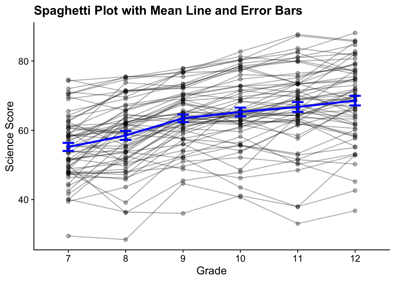
24.2.2 Unconditional Growth Mixture Model
This MplusAutomation code loops through the class-specific statements to include freeing variances and covariances.
gmm_6 <- lapply(1:6, function(k){

  # This MODEL section changes the model specification
  MODEL <- paste(sapply(1:k, function(i) {
    glue("
    %c#{i}%
    s WITH I;      ! covariances are freely estimated
    sci7-sci12;    ! variances are freely estimated
    ")
  }), collapse = "\n")

  gmm_enum  <- mplusObject(
    TITLE = glue("GMM {k}-Class"),

    VARIABLE = glue(
    "usevar = sci7-sci12;
     classes = c({k}); "),

  ANALYSIS =
   "estimator = mlr;
    type = mixture;
    starts = 200 100;
    processors = 12;",

    MODEL = glue("%OVERALL%
       i s | sci7@0 sci8@1 sci9@2 sci10@3 sci11@4 sci12@5;

       {MODEL}"), # The `MODEL` object is placed here.

    OUTPUT = "tech1 tech11 tech14 sampstat standardized svalues;",

  SAVEDATA =
    glue("FILE IS savedata_c{k}.dat;
     SAVE = cprobabilities;"),

  PLOT = "type=plot3;
          series = sci7-sci12(*)",

  usevariables = colnames(lsay_sci),
  rdata = lsay_sci)

gmm_enum_fit <- mplusModeler(gmm_enum,
                            dataout=glue(here("gmm", "gmm_enum", "gmm_lsay.dat")),
                            modelout=glue(here("gmm", "gmm_enum", "c{k}_gmm_lsay.inp")) ,
                            check=TRUE, run = TRUE, hashfilename = FALSE)
})
24.2.2.1 Table of Fit
First, extract data:
output_gmm <- readModels(here("gmm","gmm_enum"), filefilter = "gmm", quiet = TRUE)

# Extract fit indices
enum_extract <- LatexSummaryTable(
  output_gmm,
  keepCols = c(
    "Title",
    "Parameters",
    "LL",
    "BIC",
    "aBIC",
    "BLRT_PValue",
    "T11_VLMR_PValue",
    "Observations"
  ),
  sortBy = "Title"
)

# Extract lowest class size
min_sizes <- map_df(names(output_gmm), ~ {
  model <- output_gmm[[.x]]
  min_size <- min(model$class_counts$modelEstimated$proportion) * 100
  tibble(Model = .x, min_cs = round(min_size, 2))
})

# Combine dataframe
combined <- cbind(enum_extract, min_sizes)

# Calculate additional fit indices
allFit <- combined %>%
  mutate(CAIC = -2 * LL + Parameters * (log(Observations) + 1)) %>%
  mutate(AWE = -2 * LL + 2 * Parameters * (log(Observations) + 1.5)) %>%
  mutate(SIC = -.5 * BIC) %>%
  mutate(expSIC = exp(SIC - max(SIC))) %>%
  mutate(BF = exp(SIC - lead(SIC))) %>%
  mutate(cmPk = expSIC / sum(expSIC)) %>%
  dplyr::select(Title, Parameters, min_cs, LL, BIC, aBIC, CAIC, AWE, BLRT_PValue, T11_VLMR_PValue, BF, cmPk) %>%
  arrange(Parameters)
Then, create table:
fit_table1 <- allFit %>%
  gt() %>%
  tab_header(title = md("**Model Fit Summary Table**")) %>%
  cols_label(
    Title = "Classes",
    Parameters = md("Par"),
    min_cs = md("Min. Class Size"),
    LL = md("*LL*"),
    T11_VLMR_PValue = "VLMR",
    BLRT_PValue = "BLRT",
    BF = md("BF"),
    cmPk = md("*cmPk*")
  ) %>%
  tab_footnote(
    footnote = md(
      "*Note.* Par = Parameters; *LL* = model log likelihood;
BIC = Bayesian information criterion;
aBIC = sample size adjusted BIC; CAIC = consistent Akaike information criterion;
AWE = approximate weight of evidence criterion;
BLRT = bootstrapped likelihood ratio test p-value;
VLMR = Vuong-Lo-Mendell-Rubin adjusted likelihood ratio test p-value;
*cmPk* = approximate correct model probability."
    ),
locations = cells_title()
  ) %>%
  tab_options(column_labels.font.weight = "bold") %>%
  fmt_number(c(3:8),
             decimals = 2) %>%
  fmt_missing(1:12,
              missing_text = "--") %>%
  fmt(
    c(9:10, 12),
    fns = function(x)
      ifelse(x < 0.001, "<.001",
             scales::number(x, accuracy = .01))
  ) %>%
  fmt(
    11,
    fns = function (x)
      ifelse(x > 100, ">100",
             scales::number(x, accuracy = .01))
  ) %>%
  tab_style(
    style = list(
      cell_text(weight = "bold")
      ),
    locations = list(cells_body(
     columns = BIC,
     row = BIC == min(BIC[c(1:6)]) # Change this to the number of classes you estimated
    ),
    cells_body(
     columns = aBIC,
     row = aBIC == min(aBIC[1:6])
    ),
    cells_body(
     columns = CAIC,
     row = CAIC == min(CAIC[1:6])
    ),
    cells_body(
     columns = AWE,
     row = AWE == min(AWE[1:6])
    ),
    cells_body(
     columns = cmPk,
     row =  cmPk == max(cmPk[1:6])
     ),
    cells_body(
     columns = BF,
     row =  BF > 10),
    cells_body(
     columns =  T11_VLMR_PValue,
     row =  ifelse(T11_VLMR_PValue < .001 & lead(T11_VLMR_PValue) > .05, T11_VLMR_PValue < .001, NA)),
    cells_body(
     columns =  BLRT_PValue,
     row =  ifelse(BLRT_PValue < .001 & lead(BLRT_PValue) > .05, BLRT_PValue < .001, NA))
  )
)

fit_table1| Model Fit Summary Table1 | |||||||||||
| Classes | Par | Min. Class Size | LL | BIC | aBIC | CAIC | AWE | BLRT | VLMR | BF | cmPk |
|---|---|---|---|---|---|---|---|---|---|---|---|
| GMM 1-Class | 11 | 100.00 | −63,865.66 | 127,826.77 | 127,791.82 | 127,837.77 | 127,955.22 | – | – | 0.00 | <.001 |
| GMM 2-Class | 21 | 40.34 | −63,370.06 | 126,922.33 | 126,855.60 | 126,943.33 | 127,167.54 | <.001 | <.001 | 0.00 | <.001 |
| GMM 3-Class | 31 | 28.75 | −63,254.48 | 126,777.95 | 126,679.44 | 126,808.95 | 127,139.93 | <.001 | 0.01 | 0.00 | <.001 |
| GMM 4-Class | 41 | 1.93 | −63,192.38 | 126,740.50 | 126,610.22 | 126,781.50 | 127,219.26 | <.001 | 0.01 | 17.80 | 0.95 |
| GMM 5-Class | 51 | 4.30 | −63,151.87 | 126,746.26 | 126,584.20 | 126,797.26 | 127,341.78 | <.001 | 0.00 | >100 | 0.05 |
| GMM 6-Class | 61 | 3.89 | −63,117.02 | 126,763.32 | 126,569.49 | 126,824.32 | 127,475.62 | <.001 | 0.04 | – | <.001 |
| 1 Note. Par = Parameters; LL = model log likelihood; BIC = Bayesian information criterion; aBIC = sample size adjusted BIC; CAIC = consistent Akaike information criterion; AWE = approximate weight of evidence criterion; BLRT = bootstrapped likelihood ratio test p-value; VLMR = Vuong-Lo-Mendell-Rubin adjusted likelihood ratio test p-value; cmPk = approximate correct model probability. | |||||||||||
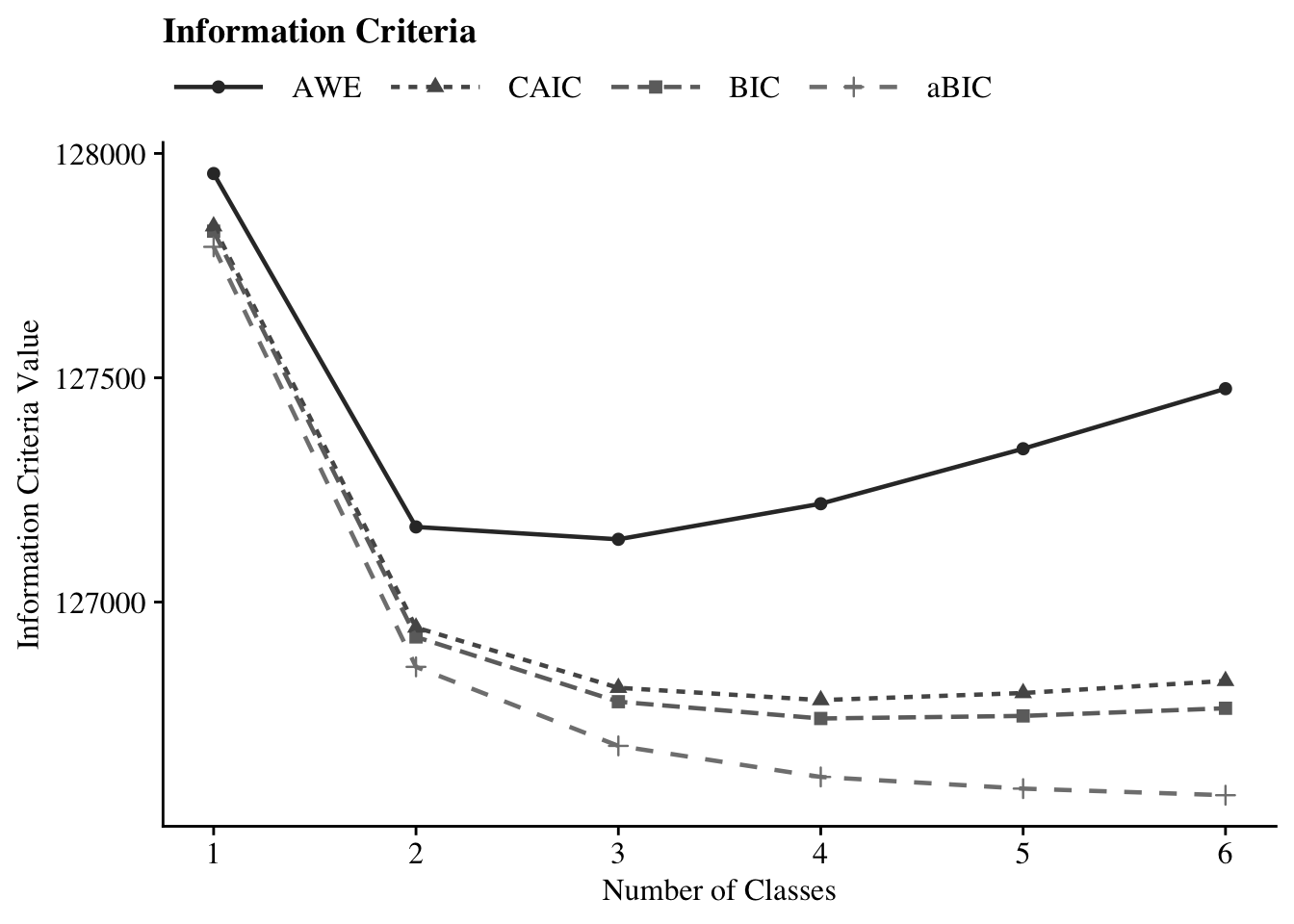
24.2.2.2 Information Criteria Plot
allFit %>%
  dplyr::select(LL:AWE) %>%
  rowid_to_column() %>%
  pivot_longer(`BIC`:`AWE`,
               names_to = "Index",
               values_to = "ic_value") %>%
  mutate(Index = factor(Index,
                        levels = c ("AWE", "CAIC", "BIC", "aBIC"))) %>%
  ggplot(aes(
    x = rowid,
    y = ic_value,
    color = Index,
    shape = Index,
    group = Index,
    lty = Index
  )) +
  geom_point(size = 2.0) + geom_line(size = .8) +
  scale_x_continuous(breaks = 1:nrow(allFit)) +
  scale_colour_grey(end = .5) +
  theme_cowplot() +
  labs(x = "Number of Classes", y = "Information Criteria Value", title = "Information Criteria") +
  theme(
    text = element_text(family = "Times", size = 12),
    legend.text = element_text(family="Times", size=12),
    legend.key.width = unit(3, "line"),
    legend.title = element_blank(),
    legend.position = "top"
  )
24.2.2.3 Plot GMM
plotGrowthMixtures(output_gmm, estimated = TRUE, rawdata = TRUE,
                   time_scale = c(1, 2, 3, 4, 5, 6), alpha_range = c(0, 0.01))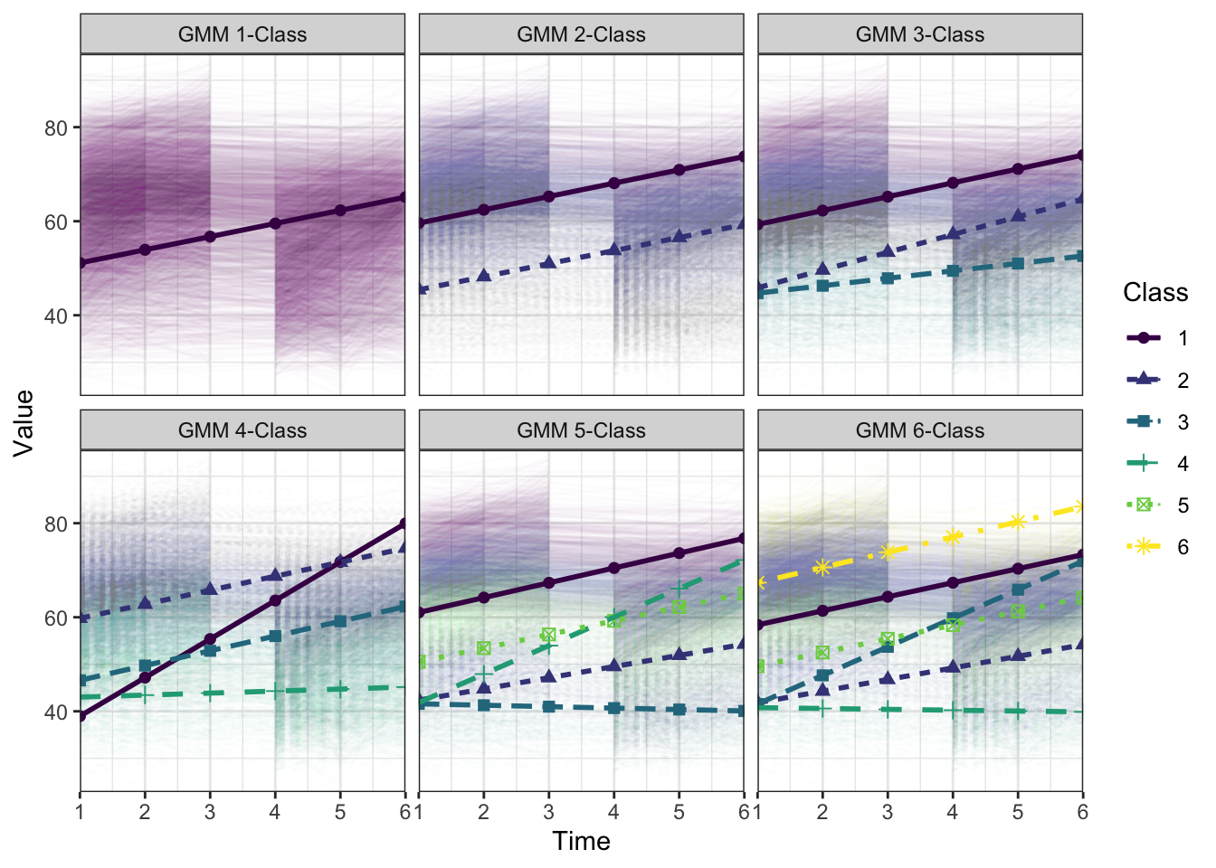
24.2.3 Covariates Growth Mixture Model
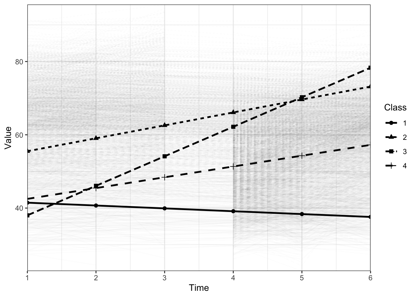
Two covariates were used in the GMM analysis and were related to the latent class variable: gender and interest in science issues in 7th grade.
step1  <- mplusObject(
  TITLE = "GMM with Covariates",
  VARIABLE =
  "usevar = sci7-sci12
  female interest7;

   classes = c(4);",

  ANALYSIS =
   "estimator = mlr;
    type = mixture;
    starts = 200 100;
    processors = 12;",

  MODEL =
    "%OVERALL%

    i s on female interest7;

    i s | sci7@0 sci8@1 sci9@2 sci10@3 sci11@4 sci12@5;

    %c#1%
    s WITH I;      ! covariances are freely estimated
    sci7-sci12;    ! variances are freely estimated
    i s on female interest7;

    %c#2%
    s WITH I;
    sci7-sci12;
    i s on female interest7;

    %c#3%
    s WITH I;
    sci7-sci12;
    i s on female interest7;

    %c#4%
    s WITH I;
    sci7-sci12;
    i s on female interest7;",

  OUTPUT = "tech1 tech11 tech14 sampstat standardized svalues;",

  SAVEDATA =
    glue("FILE IS savedata_c4.dat;
     SAVE = cprobabilities;"),

  PLOT = "type=plot3;
          series = sci7-sci12(*)",

  usevariables = colnames(lsay_sci),
  rdata = lsay_sci)

step1_fit <- mplusModeler(step1,
                            dataout=here("gmm", "gmm_cov", "gmm_cov.dat"),
                            modelout=here("gmm", "gmm_cov", "gmm_cov.inp") ,
                            check=TRUE, run = TRUE, hashfilename = FALSE)
24.2.3.1 Plot GMM
gmm_cov <- readModels(here("gmm", "gmm_cov", "gmm_cov.out"))

plotGrowthMixtures(gmm_cov, estimated = TRUE, rawdata = TRUE,
                   time_scale = c(1, 2, 3, 4, 5, 6), alpha_range = c(0, 0.01), bw = TRUE)