3 Enumeration
Example: Bullying in Schools
To demonstrate mixture modeling in the training program and online resource components of the IES grant we utilize the Civil Rights Data Collection (CRDC)8 data repository. The CRDC is a federally mandated school-level data collection effort that occurs every other year. This public data is currently available for selected latent class indicators across 4 years (2011, 2013, 2015, 2017) and all US states. In this example, we use the Arizona state sample. We utilize six focal indicators which constitute the latent class model in our example; three variables which report on harassment/bullying in schools based on disability, race, or sex, and three variables on full-time equivalent school staff hires (counselor, psychologist, law enforcement). This data source also includes covariates on a variety of subjects and distal outcomes reported in 2018 such as math/reading assessments and graduation rates.
Load packages
library(tidyverse)
library(haven)
library(glue)
library(MplusAutomation)
library(here)
library(janitor)
library(gt)
library(cowplot)
library(DiagrammeR)
3.1 Variable Description
| LCA indicators1 | ||
| Name | Label | Values |
|---|---|---|
| leaid | District Identification Code | |
| ncessch | School Identification Code | |
| report_dis | Number of students harassed or bullied on the basis of disability | 0 = No reported incidents, 1 = At least one reported incident |
| report_race | Number of students harassed or bullied on the basis of race, color, or national origin | 0 = No reported incidents, 1 = At least one reported incident |
| report_sex | Number of students harassed or bullied on the basis of sex | 0 = No reported incidents, 1 = At least one reported incident |
| counselors_fte | Number of full time equivalent counselors hired as school staff | 0 = No staff present, 1 = At least one staff present |
| psych_fte | Number of full time equivalent psychologists hired as school staff | 0 = No staff present, 1 = At least one staff present |
| law_fte | Number of full time equivalent law enforcement officers hired as school staff | 0 = No staff present, 1 = At least one staff present |
| 1 Civil Rights Data Collection (CRDC) | ||
Variables have been transformed to be dichotomous indicators using the following coding strategy
Harassment and bullying count variables are recoded 1 if the school reported at least one incident of harassment (0 indicates no reported incidents).
On the original scale reported by the CDRC staff variables for full time equivalent employees (FTE) are represented as 1 and part time employees are represented by values between 1 and 0.
Schools with greater than one staff of the designated type are represented by values greater than 1.
All values greater than zero were recorded as 1s (e.g., .5, 1,3) indicating that the school has a staff present on campus at least part time.
Schools with no staff of the designated type are indicated as 0 for the dichotomous variable.
3.2 Prepare Data
df_bully <- read_csv(here("data", "crdc_lca_data.csv")) %>%
  clean_names() %>%
  dplyr::select(report_dis, report_race, report_sex, counselors_fte, psych_fte, law_fte)
3.3 Descriptive Statistics
dframe <- df_bully %>%
pivot_longer(
c(report_dis, report_race, report_sex, counselors_fte, psych_fte, law_fte),
names_to = "Variable"
) %>%
group_by(Variable) %>%
summarise(
Count = sum(value == 1, na.rm = TRUE),
Total = n(),
.groups = "drop"
) %>%
mutate(`Proportion Endorsed` = round(Count / Total, 3)) %>%
select(Variable, `Proportion Endorsed`, Count)
gt(dframe) %>%
tab_header(
title = md("**LCA Indicator Endorsement**"),
subtitle = md(" ")
) %>%
tab_options(
column_labels.font.weight = "bold",
row_group.font.weight = "bold"
)| LCA Indicator Endorsement | ||
| Variable | Proportion Endorsed | Count |
|---|---|---|
| counselors_fte | 0.453 | 919 |
| law_fte | 0.124 | 251 |
| psych_fte | 0.467 | 947 |
| report_dis | 0.042 | 85 |
| report_race | 0.102 | 206 |
| report_sex | 0.168 | 340 |
Save as image
Frequency Plot
data_long <- df_bully %>%
  pivot_longer(c(report_dis, report_race, report_sex, counselors_fte, psych_fte, law_fte), names_to = "variable")

# Bar plot for 0/1 indicators
ggplot(data_long, aes(x = factor(value))) +
  geom_bar(fill = "#69b3a2", color = "black") +
  geom_text(stat = "count", aes(label = after_stat(count)),
            vjust = -0.5, size = 3.5) +
  facet_wrap(~ variable) +
  labs(
    title = "Binary Indicator Distributions",
    x = "Value (0 = No, 1 = Yes)",
    y = "Count"
  ) +
  theme_cowplot()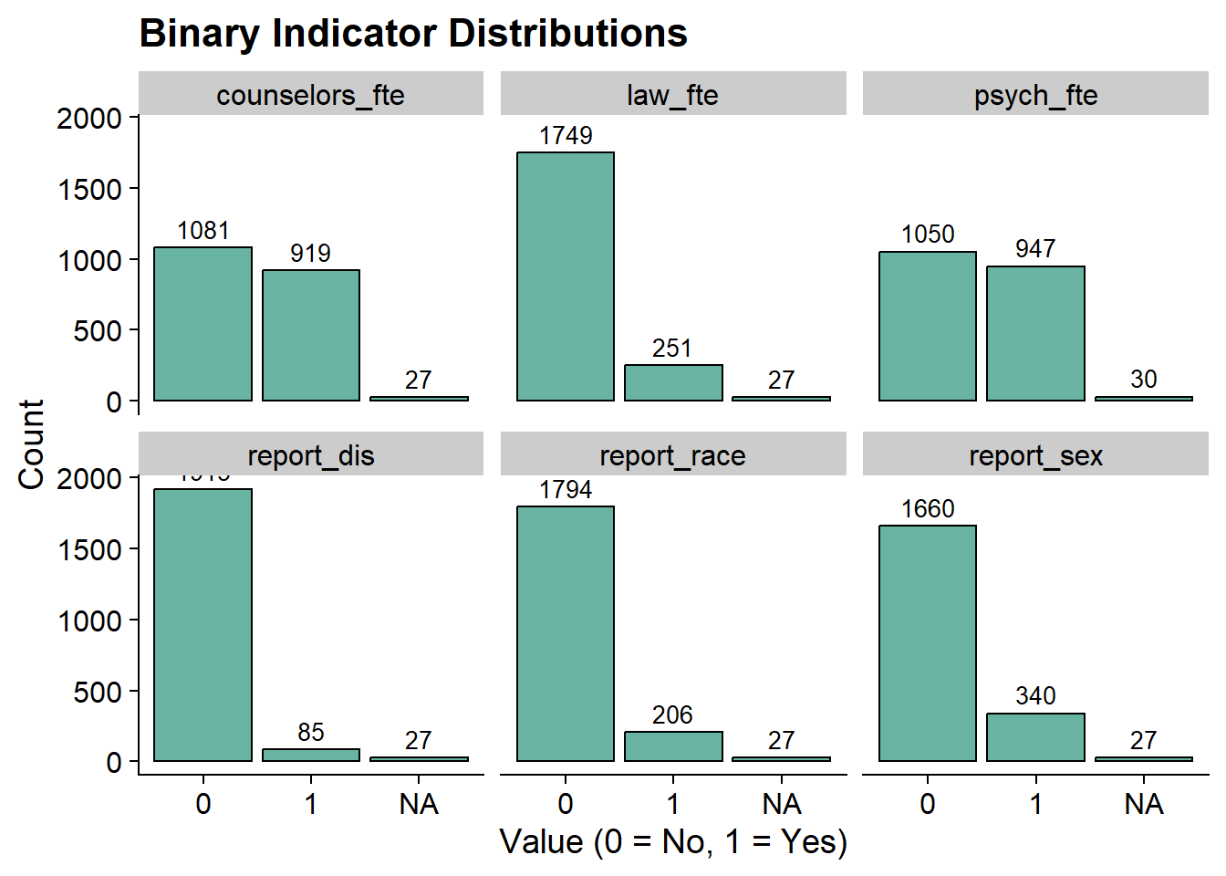
3.4 Enumeration
This code uses the mplusObject function in the MplusAutomation package and saves all model runs in the enum folder.
lca_6  <- lapply(1:6, function(k) {
  lca_enum  <- mplusObject(

    TITLE = glue("{k}-Class"),

    VARIABLE = glue(
    "categorical = report_dis-law_fte;
     usevar = report_dis-law_fte;
     classes = c({k}); "),

  ANALYSIS =
   "estimator = mlr;
    type = mixture;
    starts = 500 100;
    processors = 10;",

  OUTPUT = "sampstat residual tech11 tech14;",

  PLOT =
    "type = plot3;
    series = report_dis-law_fte(*);",

  usevariables = colnames(df_bully),
  rdata = df_bully)

lca_enum_fit <- mplusModeler(lca_enum,
                            dataout=glue(here("enum", "bully.dat")),
                            modelout=glue(here("enum", "c{k}_bully.inp")) ,
                            check=TRUE, run = TRUE, hashfilename = FALSE)
})IMPORTANT: Before moving forward, make sure to open each output document to ensure models were estimated normally.
3.5 Examine and extract Mplus files
Code by Delwin Carter (2025)
Check all Models for:
- Warnings
- Errors
- Convergence and Loglikelihood Replication Information
source(here("functions", "extract_mplus_info.R"))

# Define the directory where all of the .out files are located.
output_dir <- here("enum")

# Get all .out files
output_files <- list.files(output_dir, pattern = "\\.out$", full.names = TRUE)

# Process all .out files into one dataframe
final_data <- map_dfr(output_files, extract_mplus_info_extended)

# Extract Sample_Size from final_data
sample_size <- unique(final_data$Sample_Size)
3.5.1 Examine Mplus Warnings
Here are some of the warnings for the enumeration models for each output file corresponding to class solution.
source(here("functions", "extract_warnings.R"))

warnings_table <- extract_warnings(final_data)
warnings_table| Model Warnings | ||
| Output File | # of Warnings | Warning Message(s) |
|---|---|---|
| c1_bully.out | There are 5 warnings in the output file. | *** WARNING in VARIABLE command Note that only the first 8 characters of variable names are used in the output. Shorten variable names to avoid any confusion. |
*** WARNING in PLOT command Note that only the first 8 characters of variable names are used in plots. If variable names are not unique within the first 8 characters, problems may occur. |
||
*** WARNING in OUTPUT command SAMPSTAT option is not available when all outcomes are censored, ordered categorical, unordered categorical (nominal), count or continuous-time survival variables. Request for SAMPSTAT is ignored. |
||
*** WARNING in OUTPUT command TECH11 option is not available for TYPE=MIXTURE with only one class. Request for TECH11 is ignored. |
||
*** WARNING in OUTPUT command TECH14 option is not available for TYPE=MIXTURE with only one class. Request for TECH14 is ignored. |
||
| c2_bully.out | There are 3 warnings in the output file. | *** WARNING in VARIABLE command Note that only the first 8 characters of variable names are used in the output. Shorten variable names to avoid any confusion. |
*** WARNING in PLOT command Note that only the first 8 characters of variable names are used in plots. If variable names are not unique within the first 8 characters, problems may occur. |
||
*** WARNING in OUTPUT command SAMPSTAT option is not available when all outcomes are censored, ordered categorical, unordered categorical (nominal), count or continuous-time survival variables. Request for SAMPSTAT is ignored. |
||
| c3_bully.out | There are 3 warnings in the output file. | *** WARNING in VARIABLE command Note that only the first 8 characters of variable names are used in the output. Shorten variable names to avoid any confusion. |
*** WARNING in PLOT command Note that only the first 8 characters of variable names are used in plots. If variable names are not unique within the first 8 characters, problems may occur. |
||
*** WARNING in OUTPUT command SAMPSTAT option is not available when all outcomes are censored, ordered categorical, unordered categorical (nominal), count or continuous-time survival variables. Request for SAMPSTAT is ignored. |
||
| c4_bully.out | There are 3 warnings in the output file. | *** WARNING in VARIABLE command Note that only the first 8 characters of variable names are used in the output. Shorten variable names to avoid any confusion. |
*** WARNING in PLOT command Note that only the first 8 characters of variable names are used in plots. If variable names are not unique within the first 8 characters, problems may occur. |
||
*** WARNING in OUTPUT command SAMPSTAT option is not available when all outcomes are censored, ordered categorical, unordered categorical (nominal), count or continuous-time survival variables. Request for SAMPSTAT is ignored. |
||
| c5_bully.out | There are 3 warnings in the output file. | *** WARNING in VARIABLE command Note that only the first 8 characters of variable names are used in the output. Shorten variable names to avoid any confusion. |
*** WARNING in PLOT command Note that only the first 8 characters of variable names are used in plots. If variable names are not unique within the first 8 characters, problems may occur. |
||
*** WARNING in OUTPUT command SAMPSTAT option is not available when all outcomes are censored, ordered categorical, unordered categorical (nominal), count or continuous-time survival variables. Request for SAMPSTAT is ignored. |
||
| c6_bully.out | There are 3 warnings in the output file. | *** WARNING in VARIABLE command Note that only the first 8 characters of variable names are used in the output. Shorten variable names to avoid any confusion. |
*** WARNING in PLOT command Note that only the first 8 characters of variable names are used in plots. If variable names are not unique within the first 8 characters, problems may occur. |
||
*** WARNING in OUTPUT command SAMPSTAT option is not available when all outcomes are censored, ordered categorical, unordered categorical (nominal), count or continuous-time survival variables. Request for SAMPSTAT is ignored. |
||
# Save the warnings table
#gtsave(warnings_table, here("figures", "warnings_table.png"))
3.5.2 Examine Mplus Errors
Here are the errors for the enumeration models for each output file corresponding to class solution.
source(here("functions", "error_visualization.R"))

# Process errors
error_table_data <- process_error_data(final_data)
error_table_data| Model Estimation Errors | ||
| Output File | Model Type | Error Message |
|---|---|---|
| c2_bully.out | 2-Class | THE BEST LOGLIKELIHOOD VALUE HAS BEEN REPLICATED. RERUN WITH AT LEAST TWICE THE RANDOM STARTS TO CHECK THAT THE BEST LOGLIKELIHOOD IS STILL OBTAINED AND REPLICATED. |
| c3_bully.out | 3-Class | THE BEST LOGLIKELIHOOD VALUE HAS BEEN REPLICATED. RERUN WITH AT LEAST TWICE THE RANDOM STARTS TO CHECK THAT THE BEST LOGLIKELIHOOD IS STILL OBTAINED AND REPLICATED. IN THE OPTIMIZATION, ONE OR MORE LOGIT THRESHOLDS APPROACHED EXTREME VALUES OF -15.000 AND 15.000 AND WERE FIXED TO STABILIZE MODEL ESTIMATION. THESE VALUES IMPLY PROBABILITIES OF 0 AND 1. IN THE MODEL RESULTS SECTION, THESE PARAMETERS HAVE 0 STANDARD ERRORS AND 999 IN THE Z-SCORE AND P-VALUE COLUMNS. |
| c4_bully.out | 4-Class | THE BEST LOGLIKELIHOOD VALUE HAS BEEN REPLICATED. RERUN WITH AT LEAST TWICE THE RANDOM STARTS TO CHECK THAT THE BEST LOGLIKELIHOOD IS STILL OBTAINED AND REPLICATED. IN THE OPTIMIZATION, ONE OR MORE LOGIT THRESHOLDS APPROACHED EXTREME VALUES OF -15.000 AND 15.000 AND WERE FIXED TO STABILIZE MODEL ESTIMATION. THESE VALUES IMPLY PROBABILITIES OF 0 AND 1. IN THE MODEL RESULTS SECTION, THESE PARAMETERS HAVE 0 STANDARD ERRORS AND 999 IN THE Z-SCORE AND P-VALUE COLUMNS. |
| c5_bully.out | 5-Class | THE BEST LOGLIKELIHOOD VALUE HAS BEEN REPLICATED. RERUN WITH AT LEAST TWICE THE RANDOM STARTS TO CHECK THAT THE BEST LOGLIKELIHOOD IS STILL OBTAINED AND REPLICATED. IN THE OPTIMIZATION, ONE OR MORE LOGIT THRESHOLDS APPROACHED EXTREME VALUES OF -15.000 AND 15.000 AND WERE FIXED TO STABILIZE MODEL ESTIMATION. THESE VALUES IMPLY PROBABILITIES OF 0 AND 1. IN THE MODEL RESULTS SECTION, THESE PARAMETERS HAVE 0 STANDARD ERRORS AND 999 IN THE Z-SCORE AND P-VALUE COLUMNS. |
| c6_bully.out | 6-Class | THE BEST LOGLIKELIHOOD VALUE HAS BEEN REPLICATED. RERUN WITH AT LEAST TWICE THE RANDOM STARTS TO CHECK THAT THE BEST LOGLIKELIHOOD IS STILL OBTAINED AND REPLICATED. IN THE OPTIMIZATION, ONE OR MORE LOGIT THRESHOLDS APPROACHED EXTREME VALUES OF -15.000 AND 15.000 AND WERE FIXED TO STABILIZE MODEL ESTIMATION. THESE VALUES IMPLY PROBABILITIES OF 0 AND 1. IN THE MODEL RESULTS SECTION, THESE PARAMETERS HAVE 0 STANDARD ERRORS AND 999 IN THE Z-SCORE AND P-VALUE COLUMNS. |
# Save the errors table
#gtsave(error_table, here("figures", "error_table.png"))
3.5.3 Examine Convergence and Loglikelihood Replications
This table examines the convergence of each model based on loglikelihood replications.
source(here("functions", "summary_table.R"))

# Print Table with Superheader & Heatmap
summary_table <- create_flextable(final_data, sample_size)
summary_table
N = 2027 |
Random Starts |
Final starting value sets converging |
LL Replication |
Smallest Class |
||||||
|---|---|---|---|---|---|---|---|---|---|---|
Model |
Best LL |
npar |
Initial |
Final |
f |
% |
f |
% |
f |
% |
1-Class |
-5,443.409 |
6 |
500 |
100 |
100 |
100% |
100 |
100.0% |
2,027 |
100.0% |
2-Class |
-5,194.136 |
13 |
500 |
100 |
86 |
86% |
86 |
100.0% |
444 |
21.9% |
3-Class |
-5,122.478 |
20 |
500 |
100 |
94 |
94% |
94 |
100.0% |
216 |
10.6% |
4-Class |
-5,111.757 |
27 |
500 |
100 |
54 |
54% |
19 |
35.2% |
212 |
10.5% |
5-Class |
-5,105.589 |
34 |
500 |
100 |
38 |
38% |
6 |
15.8% |
43 |
2.1% |
6-Class |
-5,099.881 |
41 |
500 |
100 |
36 |
36% |
6 |
16.7% |
36 |
1.8% |
# Save the flextable as a PNG image
#invisible(save_as_image(summary_table, path = here("figures", "housekeeping.png")))
3.5.4 Check for Loglikelihood Replication
Visualize and examine loglikelihood replication values for each ouput file individually
# Load the function for separate plots
source(here("functions", "ll_replication_plots.R"))

# Generate individual log-likelihood replication tables
ll_replication_tables <- generate_ll_replication_plots(final_data)
ll_replication_tables| Log Likelihood Replications: 1-Class | ||
| Source File: c1_bully.out | ||
| Log Likelihood | Replication Count | % of Valid Replications |
|---|---|---|
| −5,443.409 | 100.000 | 100.00% |
| Log Likelihood Replications: 2-Class | ||
| Source File: c2_bully.out | ||
| Log Likelihood | Replication Count | % of Valid Replications |
|---|---|---|
| −5,194.136 | 86.000 | 100.00% |
| Log Likelihood Replications: 3-Class | ||
| Source File: c3_bully.out | ||
| Log Likelihood | Replication Count | % of Valid Replications |
|---|---|---|
| −5,122.478 | 94.000 | 100.00% |
| Log Likelihood Replications: 4-Class | ||
| Source File: c4_bully.out | ||
| Log Likelihood | Replication Count | % of Valid Replications |
|---|---|---|
| −5,111.757 | 19.000 | 35.19% |
| −5,111.759 | 4.000 | 7.41% |
| −5,112.253 | 5.000 | 9.26% |
| −5,113.910 | 1.000 | 1.85% |
| −5,115.532 | 17.000 | 31.48% |
| −5,115.538 | 1.000 | 1.85% |
| −5,116.981 | 3.000 | 5.56% |
| −5,117.829 | 2.000 | 3.70% |
| −5,117.837 | 2.000 | 3.70% |
| Log Likelihood Replications: 5-Class | ||
| Source File: c5_bully.out | ||
| Log Likelihood | Replication Count | % of Valid Replications |
|---|---|---|
| −5,105.589 | 6.000 | 15.79% |
| −5,105.661 | 1.000 | 2.63% |
| −5,105.791 | 3.000 | 7.89% |
| −5,105.799 | 3.000 | 7.89% |
| −5,106.628 | 1.000 | 2.63% |
| −5,106.748 | 1.000 | 2.63% |
| −5,106.864 | 1.000 | 2.63% |
| −5,106.975 | 1.000 | 2.63% |
| −5,106.983 | 1.000 | 2.63% |
| −5,107.172 | 4.000 | 10.53% |
| −5,107.449 | 1.000 | 2.63% |
| −5,107.450 | 2.000 | 5.26% |
| −5,107.458 | 1.000 | 2.63% |
| −5,107.728 | 1.000 | 2.63% |
| −5,107.958 | 1.000 | 2.63% |
| −5,108.003 | 1.000 | 2.63% |
| −5,108.058 | 1.000 | 2.63% |
| −5,108.860 | 3.000 | 7.89% |
| −5,109.002 | 1.000 | 2.63% |
| −5,110.373 | 1.000 | 2.63% |
| −5,110.474 | 1.000 | 2.63% |
| −5,111.532 | 1.000 | 2.63% |
| −5,112.695 | 1.000 | 2.63% |
| Log Likelihood Replications: 6-Class | ||
| Source File: c6_bully.out | ||
| Log Likelihood | Replication Count | % of Valid Replications |
|---|---|---|
| −5,099.881 | 6.000 | 16.67% |
| −5,100.272 | 1.000 | 2.78% |
| −5,100.780 | 1.000 | 2.78% |
| −5,100.874 | 1.000 | 2.78% |
| −5,100.928 | 2.000 | 5.56% |
| −5,101.017 | 1.000 | 2.78% |
| −5,101.071 | 3.000 | 8.33% |
| −5,101.089 | 1.000 | 2.78% |
| −5,101.332 | 1.000 | 2.78% |
| −5,101.448 | 1.000 | 2.78% |
| −5,101.494 | 1.000 | 2.78% |
| −5,101.502 | 2.000 | 5.56% |
| −5,101.512 | 1.000 | 2.78% |
| −5,101.579 | 2.000 | 5.56% |
| −5,101.859 | 1.000 | 2.78% |
| −5,101.923 | 1.000 | 2.78% |
| −5,101.964 | 1.000 | 2.78% |
| −5,102.075 | 1.000 | 2.78% |
| −5,102.275 | 1.000 | 2.78% |
| −5,102.613 | 1.000 | 2.78% |
| −5,102.616 | 1.000 | 2.78% |
| −5,103.084 | 1.000 | 2.78% |
| −5,104.611 | 1.000 | 2.78% |
| −5,106.123 | 1.000 | 2.78% |
| −5,106.486 | 1.000 | 2.78% |
| −5,107.624 | 1.000 | 2.78% |
Optionally, visualize and examine loglikelihood replication for each output file together.
ll_replication_table_all <- source(here("functions", "ll_replication_processing.R"), local = TRUE)$value
ll_replication_table_all
1-Class |
2-Class |
3-Class |
4-Class |
5-Class |
6-Class |
||||||||||||
|---|---|---|---|---|---|---|---|---|---|---|---|---|---|---|---|---|---|
LL |
N |
% |
LL |
N |
% |
LL |
N |
% |
LL |
N |
% |
LL |
N |
% |
LL |
N |
% |
-5443.409 |
100 |
100 |
-5194.136 |
86 |
100 |
-5122.478 |
94 |
100 |
-5111.757 |
19 |
35.2 |
-5105.589 |
6 |
15.8 |
-5,099.881 |
6 |
16.7 |
— |
— |
— |
— |
— |
— |
— |
— |
— |
-5111.759 |
4 |
7.4 |
-5105.661 |
1 |
2.6 |
-5,100.272 |
1 |
2.8 |
— |
— |
— |
— |
— |
— |
— |
— |
— |
-5112.253 |
5 |
9.3 |
-5105.791 |
3 |
7.9 |
-5,100.780 |
1 |
2.8 |
— |
— |
— |
— |
— |
— |
— |
— |
— |
-5113.91 |
1 |
1.9 |
-5105.799 |
3 |
7.9 |
-5,100.874 |
1 |
2.8 |
— |
— |
— |
— |
— |
— |
— |
— |
— |
-5115.532 |
17 |
31.5 |
-5106.628 |
1 |
2.6 |
-5,100.928 |
2 |
5.6 |
— |
— |
— |
— |
— |
— |
— |
— |
— |
-5115.538 |
1 |
1.9 |
-5106.748 |
1 |
2.6 |
-5,101.017 |
1 |
2.8 |
— |
— |
— |
— |
— |
— |
— |
— |
— |
-5116.981 |
3 |
5.6 |
-5106.864 |
1 |
2.6 |
-5,101.071 |
3 |
8.3 |
— |
— |
— |
— |
— |
— |
— |
— |
— |
-5117.829 |
2 |
3.7 |
-5106.975 |
1 |
2.6 |
-5,101.089 |
1 |
2.8 |
— |
— |
— |
— |
— |
— |
— |
— |
— |
-5117.837 |
2 |
3.7 |
-5106.983 |
1 |
2.6 |
-5,101.332 |
1 |
2.8 |
— |
— |
— |
— |
— |
— |
— |
— |
— |
— |
— |
— |
-5107.172 |
4 |
10.5 |
-5,101.448 |
1 |
2.8 |
— |
— |
— |
— |
— |
— |
— |
— |
— |
— |
— |
— |
-5107.449 |
1 |
2.6 |
-5,101.494 |
1 |
2.8 |
— |
— |
— |
— |
— |
— |
— |
— |
— |
— |
— |
— |
-5107.45 |
2 |
5.3 |
-5,101.502 |
2 |
5.6 |
— |
— |
— |
— |
— |
— |
— |
— |
— |
— |
— |
— |
-5107.458 |
1 |
2.6 |
-5,101.512 |
1 |
2.8 |
— |
— |
— |
— |
— |
— |
— |
— |
— |
— |
— |
— |
-5107.728 |
1 |
2.6 |
-5,101.579 |
2 |
5.6 |
— |
— |
— |
— |
— |
— |
— |
— |
— |
— |
— |
— |
-5107.958 |
1 |
2.6 |
-5,101.859 |
1 |
2.8 |
— |
— |
— |
— |
— |
— |
— |
— |
— |
— |
— |
— |
-5108.003 |
1 |
2.6 |
-5,101.923 |
1 |
2.8 |
— |
— |
— |
— |
— |
— |
— |
— |
— |
— |
— |
— |
-5108.058 |
1 |
2.6 |
-5,101.964 |
1 |
2.8 |
— |
— |
— |
— |
— |
— |
— |
— |
— |
— |
— |
— |
-5108.86 |
3 |
7.9 |
-5,102.075 |
1 |
2.8 |
— |
— |
— |
— |
— |
— |
— |
— |
— |
— |
— |
— |
-5109.002 |
1 |
2.6 |
-5,102.275 |
1 |
2.8 |
— |
— |
— |
— |
— |
— |
— |
— |
— |
— |
— |
— |
-5110.373 |
1 |
2.6 |
-5,102.613 |
1 |
2.8 |
— |
— |
— |
— |
— |
— |
— |
— |
— |
— |
— |
— |
-5110.474 |
1 |
2.6 |
-5,102.616 |
1 |
2.8 |
— |
— |
— |
— |
— |
— |
— |
— |
— |
— |
— |
— |
-5111.532 |
1 |
2.6 |
-5,103.084 |
1 |
2.8 |
— |
— |
— |
— |
— |
— |
— |
— |
— |
— |
— |
— |
-5112.695 |
1 |
2.6 |
-5,104.611 |
1 |
2.8 |
— |
— |
— |
— |
— |
— |
— |
— |
— |
— |
— |
— |
— |
— |
— |
-5,106.123 |
1 |
2.8 |
— |
— |
— |
— |
— |
— |
— |
— |
— |
— |
— |
— |
— |
— |
— |
-5,106.486 |
1 |
2.8 |
— |
— |
— |
— |
— |
— |
— |
— |
— |
— |
— |
— |
— |
— |
— |
-5,107.624 |
1 |
2.8 |

3.6 Table of Fit
First, extract data:
output_enum <- readModels(here("enum"), filefilter = "bully", quiet = TRUE)

# Extract fit indices
enum_extract <- LatexSummaryTable(
  output_enum,
  keepCols = c(
    "Title",
    "Parameters",
    "LL",
    "BIC",
    "aBIC",
    "BLRT_PValue",
    "T11_VLMR_PValue",
    "Observations"
  ),
  sortBy = "Title"
)

# Calculate additional fit indices
allFit <- enum_extract %>%
  mutate(CAIC = -2 * LL + Parameters * (log(Observations) + 1)) %>%
  mutate(AWE = -2 * LL + 2 * Parameters * (log(Observations) + 1.5)) %>%
  mutate(SIC = -.5 * BIC) %>%
  mutate(expSIC = exp(SIC - max(SIC))) %>%
  mutate(BF = exp(SIC - lead(SIC))) %>%
  mutate(cmPk = expSIC / sum(expSIC)) %>%
  dplyr::select(Title, Parameters, LL, BIC, aBIC, CAIC, AWE, BLRT_PValue, T11_VLMR_PValue, BF, cmPk) %>%
  arrange(Parameters)

# Merge columns with LL replications and class size from `final_data`
merged_table <- allFit %>%
  mutate(Title = str_trim(Title)) %>%
  left_join(
    final_data %>%
      select(
        Class_Model,
        Perc_Convergence,
        Replicated_LL_Perc,
        Smallest_Class,
        Smallest_Class_Perc
      ),
    by = c("Title" = "Class_Model")
  ) %>%
  mutate(Smallest_Class = coalesce(Smallest_Class, final_data$Smallest_Class[match(Title, final_data$Class_Model)])) %>%
  relocate(Perc_Convergence, Replicated_LL_Perc, .after = LL) %>%
  mutate(Smallest_Class_Combined = paste0(Smallest_Class, "\u00A0(", Smallest_Class_Perc, "%)")) %>%
  select(
    Title,
    Parameters,
    LL,
    Perc_Convergence,
    Replicated_LL_Perc,
    BIC,
    aBIC,
    CAIC,
    AWE,
    T11_VLMR_PValue,
    BLRT_PValue,
    Smallest_Class_Combined,
    BF,
    cmPk
  )
Then, create table:
fit_table1 <- merged_table %>%
  select(Title, Parameters, LL, Perc_Convergence, Replicated_LL_Perc,
         BIC, aBIC, CAIC, AWE,
         T11_VLMR_PValue, BLRT_PValue,
         Smallest_Class_Combined) %>%
  gt() %>%
  tab_header(title = md("**Model Fit Summary Table**")) %>%
  tab_spanner(label = "Model Fit Indices", columns = c(BIC, aBIC, CAIC, AWE)) %>%
  tab_spanner(label = "LRTs", columns = c(T11_VLMR_PValue, BLRT_PValue)) %>%
  tab_spanner(label = md("Smallest\u00A0Class"), columns = c(Smallest_Class_Combined)) %>%
  cols_label(
    Title = "Classes",
    Parameters = md("Par"),
    LL = md("*LL*"),
    Perc_Convergence = "% Converged",
    Replicated_LL_Perc = "% Replicated",
    BIC = "BIC",
    aBIC = "aBIC",
    CAIC = "CAIC",
    AWE = "AWE",
    T11_VLMR_PValue = "VLMR",
    BLRT_PValue = "BLRT",
    Smallest_Class_Combined = "n (%)"
  ) %>%
  tab_footnote(
    footnote = md(
      "*Note.* Par = Parameters; *LL* = model log likelihood;
BIC = Bayesian information criterion;
aBIC = sample size adjusted BIC; CAIC = consistent Akaike information criterion;
AWE = approximate weight of evidence criterion;
BLRT = bootstrapped likelihood ratio test p-value;
VLMR = Vuong-Lo-Mendell-Rubin adjusted likelihood ratio test p-value;
*cmPk* = approximate correct model probability."
    ),
locations = cells_title()
  ) %>%
  tab_options(column_labels.font.weight = "bold") %>%
  fmt_number(
    columns = c(3, 6:9),
    decimals = 2
  ) %>%
  sub_missing(1:11,
              missing_text = "--") %>%
  fmt(
    c(T11_VLMR_PValue, BLRT_PValue),
    fns = function(x)
      ifelse(x < 0.001, "<.001",
             scales::number(x, accuracy = .01))
  ) %>%
  fmt_percent(
    columns = c(Perc_Convergence, Replicated_LL_Perc),
    decimals = 0,
    scale_values = FALSE
  ) %>%

  cols_align(align = "center", columns = everything()) %>%
  tab_style(
    style = list(cell_text(weight = "bold")),
    locations = list(
      cells_body(columns = BIC, row = BIC == min(BIC)),
      cells_body(columns = aBIC, row = aBIC == min(aBIC)),
      cells_body(columns = CAIC, row = CAIC == min(CAIC)),
      cells_body(columns = AWE, row = AWE == min(AWE)),
      cells_body(columns = T11_VLMR_PValue,
                 row = ifelse(T11_VLMR_PValue < .05 & lead(T11_VLMR_PValue) > .05, T11_VLMR_PValue < .05, NA)),
      cells_body(columns = BLRT_PValue,
                 row = ifelse(BLRT_PValue < .05 & lead(BLRT_PValue) > .05, BLRT_PValue < .05, NA))
    )
  )

fit_table1| Model Fit Summary Table1 | |||||||||||
| Classes | Par | LL | % Converged | % Replicated |
Model Fit Indices
|
LRTs
|
Smallest Class
|
||||
|---|---|---|---|---|---|---|---|---|---|---|---|
| BIC | aBIC | CAIC | AWE | VLMR | BLRT | n (%) | |||||
| 1-Class | 6 | −5,443.41 | 100% | 100% | 10,932.50 | 10,913.44 | 10,938.50 | 10,996.19 | – | – | 2027 (100%) |
| 2-Class | 13 | −5,194.14 | 86% | 100% | 10,487.26 | 10,445.96 | 10,500.26 | 10,625.24 | <.001 | <.001 | 444 (21.9%) |
| 3-Class | 20 | −5,122.48 | 94% | 100% | 10,397.24 | 10,333.70 | 10,417.24 | 10,609.53 | <.001 | <.001 | 216 (10.6%) |
| 4-Class | 27 | −5,111.76 | 54% | 35% | 10,429.10 | 10,343.32 | 10,456.10 | 10,715.69 | 0.01 | 0.03 | 212 (10.5%) |
| 5-Class | 34 | −5,105.59 | 38% | 16% | 10,470.07 | 10,362.04 | 10,504.06 | 10,830.95 | 0.18 | 0.38 | 43 (2.1%) |
| 6-Class | 41 | −5,099.88 | 36% | 17% | 10,511.95 | 10,381.69 | 10,552.95 | 10,947.14 | 0.18 | 0.21 | 36 (1.8%) |
| 1 Note. Par = Parameters; LL = model log likelihood; BIC = Bayesian information criterion; aBIC = sample size adjusted BIC; CAIC = consistent Akaike information criterion; AWE = approximate weight of evidence criterion; BLRT = bootstrapped likelihood ratio test p-value; VLMR = Vuong-Lo-Mendell-Rubin adjusted likelihood ratio test p-value; cmPk = approximate correct model probability. | |||||||||||
Save table
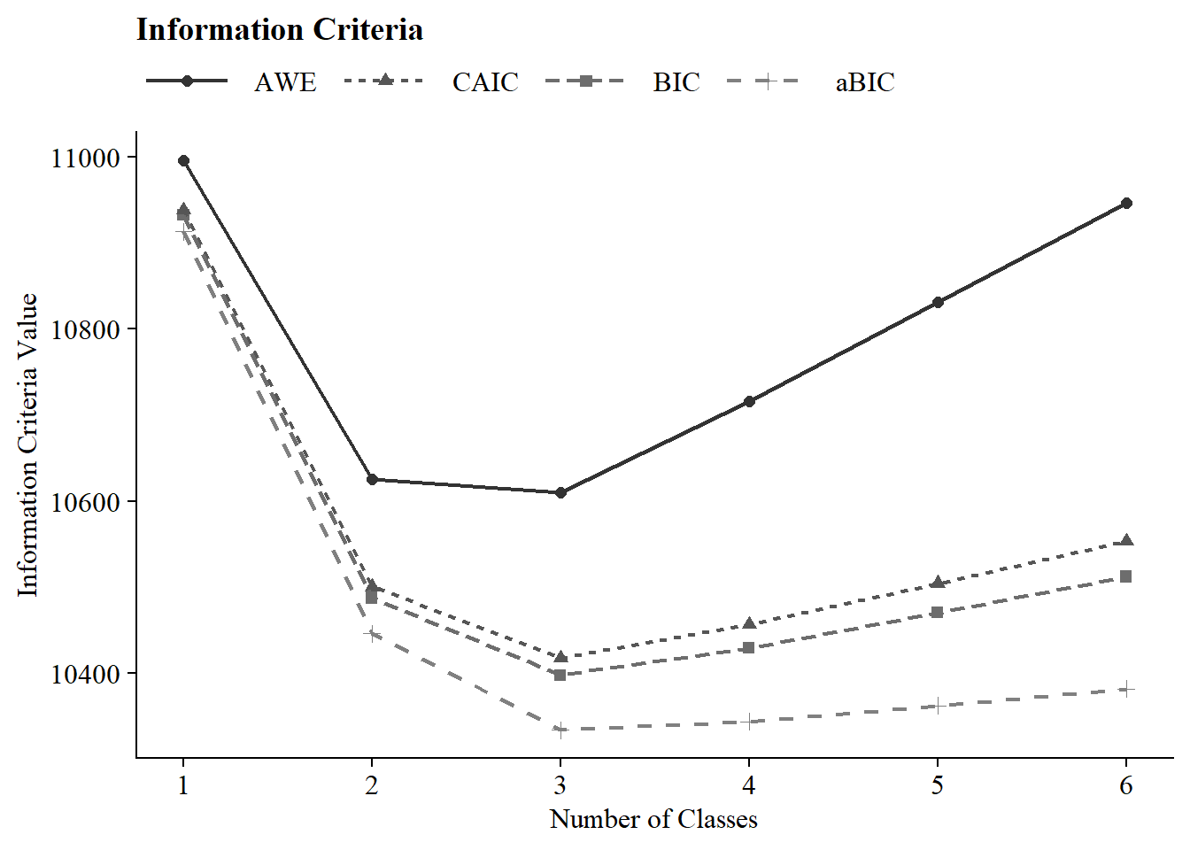
3.7 Information Criteria Plot
Below shows a Scree plot of AWE, CAIC, BIC, and aBIC summary statistics for each latent class solution.
allFit %>%
  dplyr::select(2:7) %>%
  rowid_to_column() %>%
  pivot_longer(`BIC`:`AWE`,
               names_to = "Index",
               values_to = "ic_value") %>%
  mutate(Index = factor(Index,
                        levels = c ("AWE", "CAIC", "BIC", "aBIC"))) %>%
  ggplot(aes(
    x = rowid,
    y = ic_value,
    color = Index,
    shape = Index,
    group = Index,
    lty = Index
  )) +
  geom_point(size = 2.0) + geom_line(linewidth = .8) +
  scale_x_continuous(breaks = 1:nrow(allFit)) +
  scale_colour_grey(end = .5) +
  theme_cowplot() +
  labs(x = "Number of Classes", y = "Information Criteria Value", title = "Information Criteria") +
  theme(
    text = element_text(family = "serif", size = 12),
    legend.text = element_text(family="serif", size=12),
    legend.key.width = unit(3, "line"),
    legend.title = element_blank(),
    legend.position = "top"
  )
Save figure
3.8 Compare Class Solutions
Compare probability plots for \(K = 1:6\) class solutions
model_results <- data.frame()

for (i in 1:length(output_enum)) {
  temp <- output_enum[[i]]$parameters$probability.scale %>%
    mutate(model = paste(i, "-Class Model"))

  model_results <- rbind(model_results, temp)
}

rm(temp)

compare_plot <- model_results %>%
  filter(category == 2) %>%
  dplyr::select(est, model, LatentClass, param) %>%
  mutate(param = as.factor(str_to_lower(param)),
         est = as.numeric(est))

compare_plot$param <- fct_inorder(compare_plot$param)

ggplot(
  compare_plot,
  aes(
    x = param,
    y = est,
    color = LatentClass,
    shape = LatentClass,
    group = LatentClass,
    lty = LatentClass
  )
) +
  geom_point() +
  geom_line() +
  scale_colour_viridis_d() +
  ylim(0,1) +
  facet_wrap( ~ model, ncol = 2) +
  labs(title = "Bullying Items", x = NULL, y = "Probability") +
  theme_minimal() +
  theme(panel.grid.major.y = element_blank(),
axis.text.x = element_text(angle = -45, hjust = -.1)) 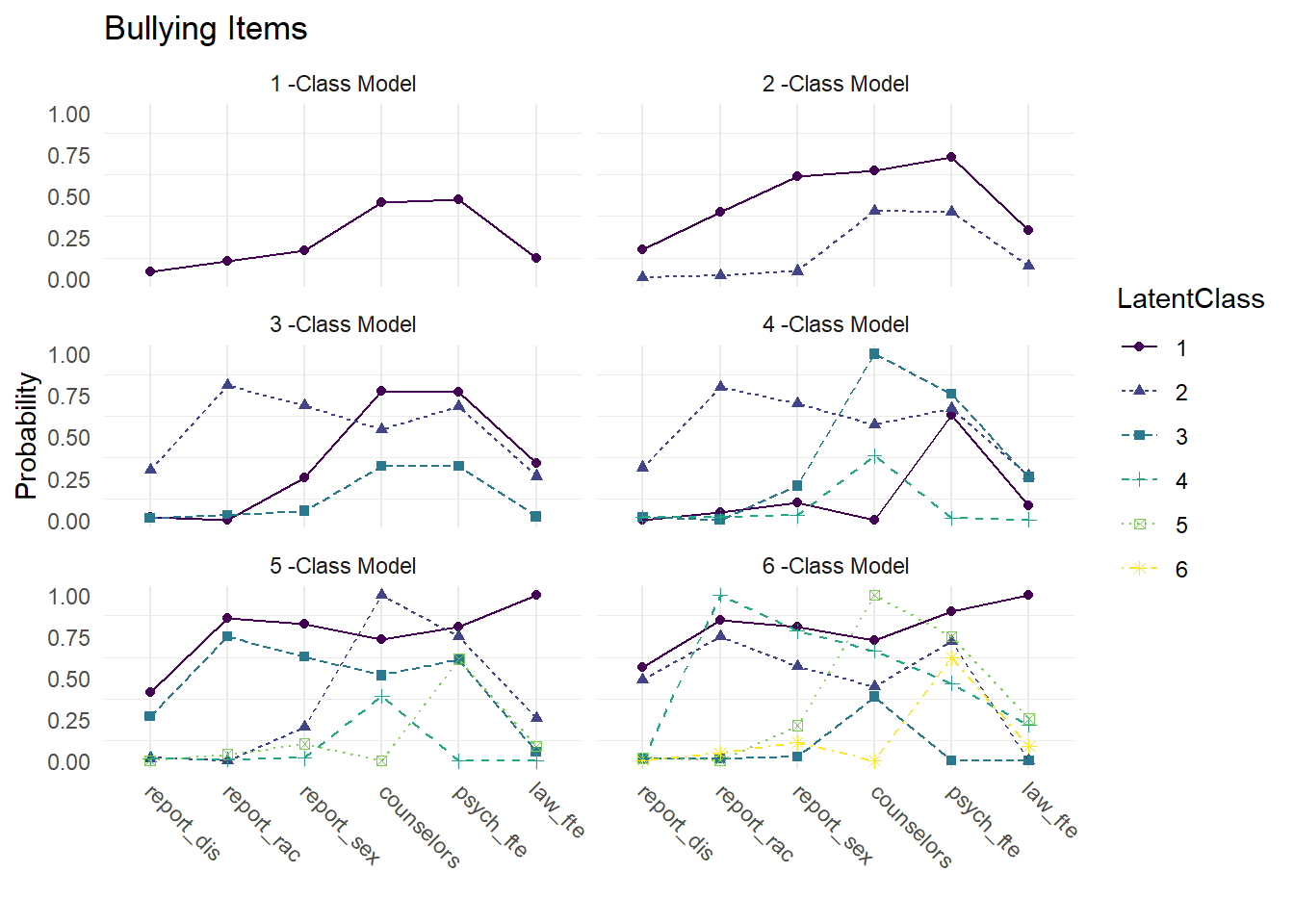
Save figure: