12 Class Separation
12.1 Load Packages
library(naniar)
library(tidyverse)
library(haven)
library(glue)
library(MplusAutomation)
library(here)
library(janitor)
library(gt)
library(tidyLPA)
library(pisaUSA15)
library(cowplot)
library(filesstrings)
library(patchwork)
library(RcppAlgos)
12.2 LCA
Continuing the LCA example (3) in this bookdown, use R to evaluate the LCA class separation.
\[\widehat{OR_{1v2}} = \frac{\frac{P(u_1=1|c_1)}{P(u_1=0|c_1)}}{\frac{P(u_1=1|c_2)}{P(u_1=0|c_2)}} \]
Odds ratios (ORs) of item endorsements between two classes >5 (corresponding to class-specific endorsement probabilities of >.7 and <.3) or <.2 (corresponding to class-specific endorsement probabilities of <.3 and >.7), indicate high separation between those two classes on that specific item. No single binary (0/1) indicator can separate more than two subsets of latent classes, no matter what the total number of classes in the model. We want a high degree of separation (large standardized mean differences) between classes.
# Read in model
output_enum <- readModels(here("enum"), filefilter = "bully", quiet = TRUE)

# Change this to look at your chosen LCA model
chosen_model <- output_enum$c4_bully.out

# Extract table of probabilities
c_prob <- data.frame(chosen_model$parameters$probability.scale) %>%
  mutate(LatentClass = sub("^", "Class ", LatentClass)) %>%
  filter(category == 2) %>%
  dplyr::select(est, LatentClass, param) %>%
  rename(item = param, prob = est, k = LatentClass) %>%
  mutate(# Adjust probabilities by setting a minimum of 0.01 and a maximum of 0.99
    prob = pmin(pmax(prob, 0.01), 0.99),
    prob = as.numeric(prob))


# Relative class sizes
class_sizes <- data.frame(chosen_model$class_counts$modelEstimated) %>%
  rename(size = proportion, k = class) %>%
  mutate(k = paste0("Class ", k)) %>%
  dplyr::select(-count)


# Create the combinations of classes
class_combinations <- data.frame(comboGrid(
  k1 = unique(class_sizes$k),
  k2 = unique(class_sizes$k)
)) %>%
  filter(k1 != k2) %>%
  arrange(k1, k2)

# Calculate pairwise comparisons for probabilities (e.g., P(u1=1|c1) / P(u1=0|c1) for each combination)
combined_results <- class_combinations %>%
  rowwise() %>%
  do({
    pair <- .
    k1 <- pair$k1
    k2 <- pair$k2

    # Filter for the probabilities (P(u1=1|c1) and P(u1=0|c1))
    data_k1_prob <- c_prob %>% filter(k == k1)
    data_k2_prob <- c_prob %>% filter(k == k2)

    # Combine the probability data for the two profiles
    prob_data <- data_k1_prob %>%
      inner_join(data_k2_prob,
                 by = "item",
                 suffix = c("_k1", "_k2")) %>%
      mutate(
        prob_ratio = (prob_k1 / (1 - prob_k1)) / (prob_k2 / (1 - prob_k2)),
        # Division formula
        comparison = paste(k1, "vs", k2)
      ) %>%
      mutate(prob_ratio = round(ifelse(
        is.infinite(prob_ratio) | is.nan(prob_ratio),
        NA,
        prob_ratio
      ), 3)) %>%
      dplyr::select(item, prob_ratio, comparison)

    prob_data
  }) %>%
  bind_rows()


# Define a function to apply the Markdown bold formatting
bold_condition <- function(x) {
  # If prob_ratio is > 5 or < 0.2, add **
  ifelse(x > 5 | x < 0.2, paste0("**", sprintf("%.3f", x), "**"),
         sprintf("%.3f", x))
}

# Assuming combined_results is already created as mentioned
formatted_results <- combined_results %>%
  dplyr::select(prob_ratio, comparison, item) %>%
  pivot_wider(names_from = comparison, values_from = prob_ratio) %>%
  mutate(across(where(is.numeric), ~ sapply(., bold_condition)))

# Create a gt table
formatted_results %>%
  gt() %>%
  cols_label(item = "Item") %>%
  fmt_missing(columns = everything(), missing_text = "-") %>%
  tab_header(title = "Class Separation Table") %>%
  fmt_markdown(columns = everything()) %>%
tab_footnote(footnote = "Cells in bold indicate probabilities > 5 or < 0.2.")| Class Separation Table | ||||||
| Item | Class 1 vs Class 2 | Class 1 vs Class 3 | Class 1 vs Class 4 | Class 2 vs Class 3 | Class 2 vs Class 4 | Class 3 vs Class 4 |
|---|---|---|---|---|---|---|
| REPORT_DIS | 28.150 | 28.150 | 45.315 | 1.000 | 1.610 | 1.610 |
| REPORT_RAC | 388.685 | 214.191 | 83.321 | 0.551 | 0.214 | 0.389 |
| REPORT_SEX | 9.018 | 90.139 | 19.912 | 9.995 | 2.208 | 0.221 |
| COUNSELORS | 0.014 | 2.161 | 133.394 | 158.812 | 9801.000 | 61.714 |
| PSYCH_FTE | 0.649 | 200.094 | 1.187 | 308.407 | 1.830 | 0.006 |
| LAW_FTE | 1.059 | 36.061 | 3.823 | 34.065 | 3.611 | 0.106 |
| Cells in bold indicate probabilities > 5 or < 0.2. | ||||||
12.3 LPA
Continuing the LPA example (7) in this bookdown, use R to evaluate the LPA profile separation.
You can evaluate the degree of profile separation by assessing the actual distance between the profile-specific means. To quantify profile separation between Profile j and Profile k with respect to a particular item m, compute a standard mean difference:
\[\hat{d}_{mjk}= \frac{{\hat{\alpha_{mj}}-\hat{\alpha_{mk}}}}{\sigma_{mjk}}\] Pooled variance:
\[\hat{\sigma}_{mj k} = \sqrt{\frac{(\hat{\pi}_j)(n)(\hat{\theta}_{mj}) + (\hat{\pi}_k)(n)(\hat{\theta}_{mk})}{(\hat{\pi}_j + \hat{\pi}_k) n}}\]
Well-separated classes have a small degree of overlap of the class-specific indicator distributions; that is, standardized mean difference is large.
A mean difference <.85 corresponds to low separation—more than 50% overlap
A mean difference > 2 corresponds to high separation—less than 20% overlap
# Read in model
output_enum <- readModels(here("lpa", "tidyLPA"), quiet = TRUE)

# Change this to look at your chosen LPA model
chosen_model <- output_enum$model_3_class_4.out

# Profile-specific means
profile_means <- data.frame(chosen_model$parameters$unstandardized) %>%
  filter(paramHeader == "Means") %>%
  filter(!str_detect(param, "#")) %>%
  dplyr::select(param, est, LatentClass) %>%
  rename(item = param,
         means = est,
         k = LatentClass) %>%
  mutate(k = paste0("Profile ", k)) %>%
  mutate(item = str_sub(item, 1, 8))

# Relative profile sizes
profile_sizes <- data.frame(chosen_model$class_counts$modelEstimated) %>%
  rename(size = proportion,
         k = class) %>%
  mutate(k = paste0("Profile ", k)) %>%
  dplyr::select(-count)

# Sample size
n <- chosen_model$summaries$Observations

# Profile-specific variance
profile_variances <- data.frame(chosen_model$parameters$unstandardized) %>%
  filter(paramHeader == "Variances") %>%
  dplyr::select(param, est, LatentClass) %>%
  rename(item = param,
         variance = est,
         k = LatentClass) %>%
  mutate(k = paste0("Profile ", k)) %>%
  mutate(item = str_sub(item, 1, 8))

# Combine profile variances with profile sizes
variance_with_sizes <- profile_variances %>%
  left_join(profile_sizes, by = "k")

# Create the combinations
profile_combinations <- data.frame(comboGrid(k1 = unique(profile_sizes$k), k2 = unique(profile_sizes$k))) %>%
  filter(k1 != k2) %>%
  arrange(k1, k2)

# Calculate pooled variance for each item across the profiles
combined_results <- profile_combinations %>%
  rowwise() %>%
  do({
    pair <- .
    k1 <- pair$k1
    k2 <- pair$k2

    # Filter for the two profiles (variance)
    data_k1_var <- variance_with_sizes %>% filter(k == k1)
    data_k2_var <- variance_with_sizes %>% filter(k == k2)

    # Filter for the two profiles (means)
    data_k1_mean <- profile_means %>% filter(k == k1)
    data_k2_mean <- profile_means %>% filter(k == k2)

    # Combine variance data for the two profiles
    variance_data <- data_k1_var %>%
      inner_join(data_k2_var, by = "item", suffix = c("_k1", "_k2")) %>%
      mutate(
        pooled_variance = sqrt(
          ((size_k1 * n * variance_k1) + (size_k2 * n * variance_k2)) / ((size_k1 + size_k2) * n)
        ),
        comparison = paste(k1, "vs", k2)
      ) %>%
      dplyr::select(item, pooled_variance, comparison)

    # Combine mean data for the two profilees
    mean_data <- data_k1_mean %>%
      inner_join(data_k2_mean, by = "item", suffix = c("_k1", "_k2")) %>%
      mutate(
        mean_diff = means_k1 - means_k2,
        comparison = paste(k1, "vs", k2)
      ) %>%
      dplyr::select(item, mean_diff, comparison)

    # Combine both variance and mean differences data
    combined_data <- variance_data %>%
      left_join(mean_data, by = c("item", "comparison")) %>%
      mutate(
         mean_diff_by_pooled_variance = mean_diff / pooled_variance
      )

    combined_data
  }) %>%
  bind_rows() %>%
  mutate(mean_diff_by_pooled_variance = round(mean_diff_by_pooled_variance, 3)) %>%
  dplyr::select(mean_diff_by_pooled_variance, comparison, item) %>%
  pivot_wider(
    names_from = comparison,
    values_from = mean_diff_by_pooled_variance
  )


# Create a gt table
gt_table <- combined_results %>%
  gt() %>%
  cols_label(
    item = "Item"
  ) %>%
  tab_header(
    title = "Profile Separation Table"
  ) %>%
  tab_footnote(
    footnote = "Green cells indicate >2; Red cells indicate <0.85."
  )


# Formatting thresholds
high_threshold <- 2
low_threshold <- 0.85


# Apply conditional colors for each numeric cell
num_cols <- gt_table$`_data` %>% dplyr::select(-item) %>% names()  # numeric columns
for(col in num_cols){
  for(i in 1:nrow(combined_results)){
    val <- combined_results[[col]][i]  # numeric value
    color <- if(val > 2) "#66BB6A" else if(val < 0.85) "#E57373" else NA
    if(!is.na(color)){
      gt_table <- gt_table %>%
        tab_style(
          style = cell_fill(color = color),
          locations = cells_body(columns = col, rows = i)
        )
    }
  }
}

# Display table
gt_table| Profile Separation Table | ||||||
| Item | Profile 1 vs Profile 2 | Profile 1 vs Profile 3 | Profile 1 vs Profile 4 | Profile 2 vs Profile 3 | Profile 2 vs Profile 4 | Profile 3 vs Profile 4 |
|---|---|---|---|---|---|---|
| BROAD_IN | -0.334 | -0.357 | 0.084 | -0.024 | 0.418 | 0.442 |
| ENJOYMEN | -0.346 | -0.722 | 0.255 | -0.375 | 0.602 | 0.977 |
| INSTRUME | 4.004 | 8.900 | -5.923 | 4.896 | -9.926 | -14.822 |
| SELF_EFF | 0.261 | 0.621 | -0.027 | 0.360 | -0.288 | -0.648 |
| Green cells indicate >2; Red cells indicate <0.85. | ||||||
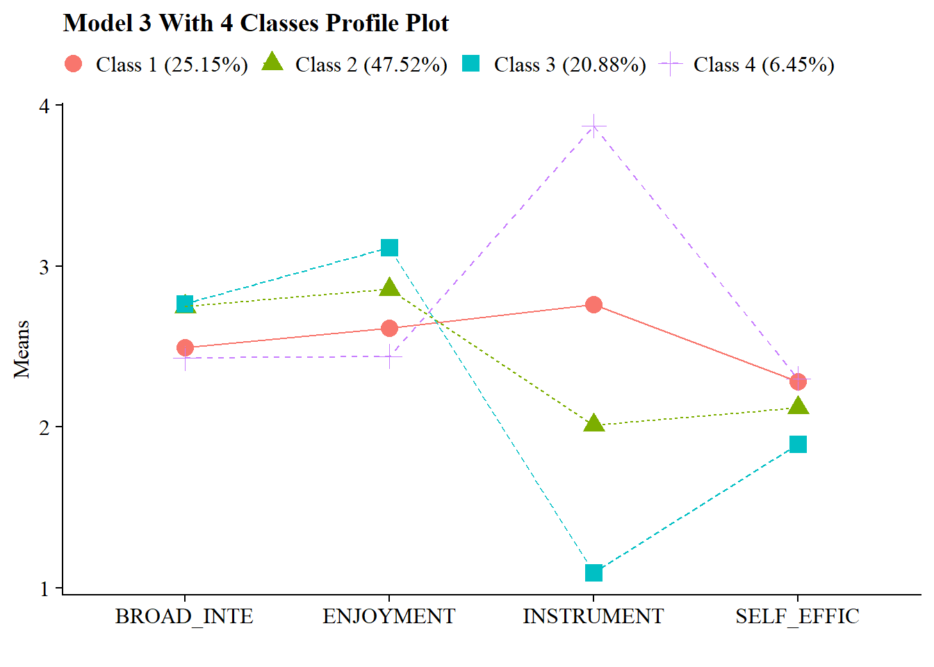
You can also visualize the plot:
source(here("functions", "plot_lpa.R"))

output_enum <- readModels(here("lpa", "tidyLPA"), quiet = TRUE)

plot_lpa(model_name = output_enum$model_3_class_4.out)