14 Manual 3-Step Distal Only

---

Data source:

1. The first examples utilizes the public-use dataset, The Longitudinal Survey of American Youth (LSAY): See documentation here

2. The second example utilizes a dataset on undergraduate Cheating available from the poLCA package (Dayton, 1998): See documentation here

---

14.1 Load packages

library(MplusAutomation)
library(tidyverse) #collection of R packages designed for data science
library(here) #helps with filepaths
library(janitor) #clean_names
library(gt) # create tables
library(cowplot) # a ggplot theme
library(DiagrammeR) # create path diagrams
library(glue) # allows us to paste expressions into R code
library(data.table) # used for `melt()` function  
library(poLCA)
library(reshape2)

---

Our example is Math IRT Score as a distal outcome of Math Attitude classes

---

Application: Longitudinal Study of American Youth, Math Attitudes

LCA Indicators & Auxiliary Variables: Math Attitudes Example
Name	Variable Description
enjoy	I enjoy math.
useful	Math is useful in everyday problems.
logical	Math helps a person think logically.
job	It is important to know math to get a good job.
adult	I will use math in many ways as an adult.
Auxiliary Variables
math_irt	Standardized IRT math test score - 12th grade.

---

The data can be found in the data folder and is called lsay_subset.csv.

lsay_data <- read_csv(here("three_step","data","lsay_subset.csv")) %>% 
  clean_names() %>%   # make variable names lowercase
  mutate(female = recode(gender, `1` = 0, `2` = 1)) # relabel values from 1,2 to 0,1

---

14.2 Descriptive Statistics

dframe <- lsay_data %>%
  pivot_longer(
    c(enjoy, useful, logical, job, adult),
    names_to = "Variable"
  ) %>%
  group_by(Variable) %>%
  summarise(
    Count = sum(value == 1, na.rm = TRUE),
    Total = n(),
    .groups = "drop"
  ) %>%
  mutate(`Proportion Endorsed` = round(Count / Total, 3)) %>%
  dplyr::select(Variable, `Proportion Endorsed`, Count)

gt(dframe) %>%
  tab_header(
    title = md("**LCA Indicator Endorsement**"),
    subtitle = md("&nbsp;")
  ) %>%
  tab_options(
    column_labels.font.weight = "bold",
    row_group.font.weight = "bold"
  )

LCA Indicator Endorsement
Variable	Proportion Endorsed	Count
adult	0.596	1858
enjoy	0.573	1784
job	0.625	1947
logical	0.541	1686
useful	0.589	1835

Math IRT Score

summary(lsay_data$math_irt)
#>    Min. 1st Qu.  Median    Mean 3rd Qu.    Max.    NA's 
#>   26.57   50.00   59.30   58.81   68.21   94.19     875

---

14.3 Manual ML Three-step

---

14.3.1 Step 1 - Class Enumeration w/ Auxiliary Specification

---

This step is done after class enumeration (or after you have selected the best latent class model). In this example, the four class model was the best. Now, we re-estimate the four-class model using optseed for efficiency. The difference here is the SAVEDATA command, where I can save the posterior probabilities and the modal class assignment that will be used in steps two and three.

step1  <- mplusObject(
  TITLE = "Step 1 - Three-Step using LSAL", 
  VARIABLE = 
  "categorical = enjoy useful logical job adult; 
   usevar = enjoy useful logical job adult;
    
   classes = c(4); 
    
   auxiliary =  math_irt  ! distal outcome ",
  
  ANALYSIS = 
   "estimator = mlr; 
    type = mixture;
    starts = 0;
    optseed = 568405;",
  
  SAVEDATA = 
   "File=savedata_dis.dat;
    Save=cprob;",
  
  OUTPUT = "residual tech11 tech14",
  
  PLOT = 
    "type = plot3; 
    series = enjoy-adult(*);",
  
  usevariables = colnames(lsay_data),
  rdata = lsay_data)

step1_fit <- mplusModeler(step1,
                            dataout=here("three_step", "manual_3step", "Step1.dat"),
                            modelout=here("three_step", "manual_3step", "one_dis.inp") ,
                            check=TRUE, run = TRUE, hashfilename = FALSE)

---

source(here("functions", "plot_lca.R"))
output_lsay <- readModels(here("three_step", "manual_3step","one_dis.out"))

plot_lca(model_name = output_lsay)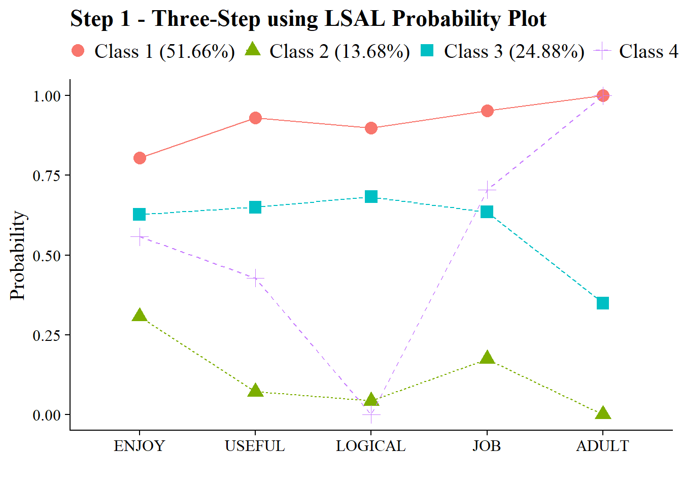

---

14.3.2 Step 2 - Determine Measurement Error

---

Extract logits for the classification probabilities for the most likely latent class

logit_cprobs <- as.data.frame(output_lsay[["class_counts"]]
                                       [["logitProbs.mostLikely"]])

Extract saved dataset which is part of the mplusObject “step1_fit”

savedata <- as.data.frame(output_lsay[["savedata"]])

Rename the column in savedata named “C” and change to “N”

colnames(savedata)[colnames(savedata)=="C"] <- "N"

---

14.3.3 Step 3 - LCA Auxiliary Variable Model with 1 Distal Outcome

---

step3  <- mplusObject(
  TITLE = "Step3 - 3step LSAY", 
  
  VARIABLE = 
 "nominal=N;
  usevar = n;
  
  classes = c(4);
  
  usevar = math_irt;" ,
  
  ANALYSIS = 
 "estimator = mlr; 
  type = mixture; 
  starts = 0;",
  
  MODEL =
  glue(
 " %OVERALL%
 

     %C#1%
  [n#1@{logit_cprobs[1,1]}]; ! MUST EDIT if you do not have a 4-class model. 
  [n#2@{logit_cprobs[1,2]}];
  [n#3@{logit_cprobs[1,3]}];
  
  [math_irt](m1);    ! conditional distal mean 
  math_irt;          ! conditional distal variance (freely estimated)

  %C#2%
  [n#1@{logit_cprobs[2,1]}];
  [n#2@{logit_cprobs[2,2]}];
  [n#3@{logit_cprobs[2,3]}];
  
  [math_irt](m2);
  math_irt;
  
  %C#3%
  [n#1@{logit_cprobs[3,1]}];
  [n#2@{logit_cprobs[3,2]}];
  [n#3@{logit_cprobs[3,3]}];
  
  [math_irt](m3);
  math_irt;

  %C#4%
  [n#1@{logit_cprobs[4,1]}];
  [n#2@{logit_cprobs[4,2]}];
  [n#3@{logit_cprobs[4,3]}];
  
  [math_irt](m4);
  math_irt; "),
  
  MODELCONSTRAINT = 
   "New (diff12 diff13 diff23 
    diff14 diff24 diff34);
  
    diff12 = m1-m2;  ! test pairwise distal mean differences
    diff13 = m1-m3;
    diff23 = m2-m3;
    diff14 = m1-m4;
    diff24 = m2-m4;
    diff34 = m3-m4;",
  
  MODELTEST = "     ! omnibus test of distal means 
    m1=m2;
    m2=m3;
    m3=m4;",
  
 
  usevariables = colnames(savedata), 
  rdata = savedata)

step3_fit <- mplusModeler(step3,
               dataout=here("three_step", "manual_3step", "Step3.dat"), 
               modelout=here("three_step", "manual_3step", "three_dis.inp"), 
               check=TRUE, run = TRUE, hashfilename = FALSE)

---

14.3.3.1 Wald Test Table

This is testing if there is a relation between the latent class variable and the distal outcome (mathirt)

modelParams <- readModels(here("three_step", "manual_3step", "three_dis.out"))

# Extract information as data frame
wald <- as.data.frame(modelParams[["summaries"]]) %>%
  dplyr::select(WaldChiSq_Value:WaldChiSq_PValue) %>% 
  mutate(WaldChiSq_DF = paste0("(", WaldChiSq_DF, ")")) %>% 
  unite(wald_test, WaldChiSq_Value, WaldChiSq_DF, sep = " ") %>% 
  rename(pval = WaldChiSq_PValue) %>% 
  mutate(pval = ifelse(pval<0.001, paste0("<.001*"),
                       ifelse(pval<0.05, paste0(scales::number(pval, accuracy = .001), "*"),
                              scales::number(pval, accuracy = .001))))

# Create table

wald_table <- wald %>% 
  gt() %>%
    tab_header(
    title = "Wald Test Distal Means (Math IRT Scores)") %>%
    cols_label(
      wald_test = md("Wald Test (*df*)"), 
      pval = md("*p*-value")) %>% 
  cols_align(align = "center") %>% 
  opt_align_table_header(align = "left") %>% 
  gt::tab_options(table.font.names = "serif")

wald_table

Wald Test Distal Means (Math IRT Scores)
Wald Test (df)	p-value
69.108 (3)	<.001*

Save figure

gtsave(wald_table, here("figures","wald_table.docx"))

---

14.3.3.2 Table of Pairwise Distal Outcome Differences

modelParams <- readModels(here("three_step", "manual_3step", "three_dis.out"))

# Extract information as data frame
diff <- as.data.frame(modelParams[["parameters"]][["unstandardized"]]) %>%
  filter(grepl("DIFF", param)) %>% 
  dplyr::select(param:pval) %>% 
  mutate(se = paste0("(", format(round(se,2), nsmall =2), ")")) %>% 
  unite(estimate, est, se, sep = " ") %>% 
  mutate(param = str_remove(param, "DIFF"),
         param = as.numeric(param)) %>% 
  separate(param, into = paste0("Group", 1:2), sep = 1) %>% 
  mutate(class = paste0("Class ", Group1, " vs ", Group2)) %>% 
  dplyr::select(class, estimate, pval) %>% 
  mutate(pval = ifelse(pval<0.001, paste0("<.001*"),
                       ifelse(pval<0.05, paste0(scales::number(pval, accuracy = .001), "*"),
                              scales::number(pval, accuracy = .001))))

# Create table

diff %>% 
  gt() %>%
    tab_header(
    title = "Distal Outcome Differences") %>%
    cols_label(
      class = "Class",
      estimate = md("Mean (*se*)"),
      pval = md("*p*-value")) %>% 
    sub_missing(1:3,
              missing_text = "") %>%
  cols_align(align = "center") %>% 
  opt_align_table_header(align = "left") %>% 
  gt::tab_options(table.font.names = "serif")

Distal Outcome Differences
Class	Mean (se)	p-value
Class 1 vs 2	6.731 (0.98)	<.001*
Class 1 vs 3	3.103 (0.96)	0.001*
Class 2 vs 3	-3.628 (1.31)	0.006*
Class 1 vs 4	7.027 (1.29)	<.001*
Class 2 vs 4	0.296 (1.45)	0.838
Class 3 vs 4	3.924 (1.49)	0.008*

---

14.3.3.3 Plot Distal Outcome Means

modelParams <- readModels(here("three_step", "manual_3step", "three_dis.out"))

# Extract class size 
c_size <- as.data.frame(modelParams[["class_counts"]][["modelEstimated"]][["proportion"]]) %>% 
  rename("cs" = 1) %>% 
  mutate(cs = round(cs*100, 2))

c_size_val <- paste0("C", 1:nrow(c_size), glue(" ({c_size[1:nrow(c_size),]}%)"))


# Extract information as data frame
estimates <- as.data.frame(modelParams[["parameters"]][["unstandardized"]]) %>%
  filter(paramHeader == "Means") %>%
  dplyr::select(param, est, se) %>% 
  filter(param == "MATH_IRT") %>% 
  mutate(across(c(est, se), as.numeric)) %>% 
  mutate(LatentClass = c_size_val)

# Add labels (NOTE: You must change the labels to match the significance testing!!) 
#value_labels <- paste0(estimates$est, c("a"," bc"," abd"," cd"))

estimates$LatentClass <- fct_inorder(estimates$LatentClass)

# Plot bar graphs
estimates %>%
  ggplot(aes(x=LatentClass, y = est, fill = LatentClass)) +
  geom_col(position = "dodge", color = "black") +
  geom_errorbar(aes(ymin=est-se, ymax=est+se),
                linewidth=.3,    # Thinner lines
                width=.2,
                position=position_dodge(.9)) +
  geom_text(aes(label = est), 
            family = "serif", size = 4,
            position=position_dodge(.9),
            vjust = 8) +  
 # scale_fill_grey(start = .4, end = .7) + # Remove for colorful bars
  labs(y="Math Scores", x="") +
  theme_cowplot() +
  theme(text = element_text(family = "serif", size = 15),
        axis.text.x = element_text(size=15),
        legend.position="none")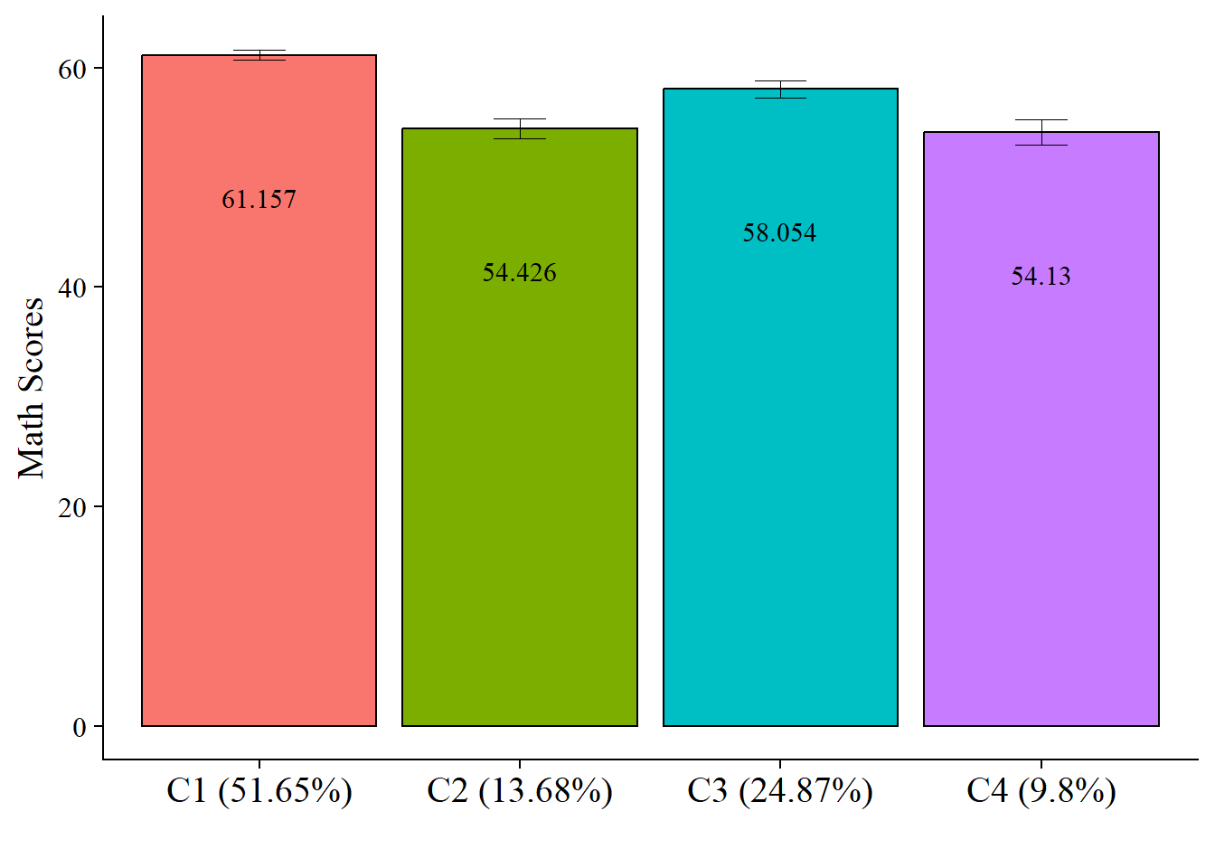

# Save plot
ggsave(here("figures","ManualDistal_Plot.jpeg"),              
       dpi=300, width=10, height = 7, units="in") 

---

14.4 Automated Three-Step

---

Application: Undergraduate Cheating behavior

“Dichotomous self-report responses by 319 undergraduates to four questions about cheating behavior” (poLCA, 2016).

---

Prepare data

data(cheating)

cheating <- cheating %>% clean_names() 

df_cheat <-  cheating %>%                                  
  dplyr::select(1:4) %>%                                  
  mutate_all(funs(.-1)) %>%                                
  mutate(gpa = cheating$gpa)

# Detaching packages that mask the dpylr functions 
detach(package:poLCA, unload = TRUE)
detach(package:MASS, unload = TRUE)

---

14.4.1 DU3STEP

DU3STEP incorporates distal outcome variables (assumed to have unequal means and variances) with mixture models.

---

---

14.4.1.1 Run the DU3step model with gpa as distal outcome

m_stepdu  <- mplusObject(
  TITLE = "DU3STEP - GPA as Distal", 
  VARIABLE = 
   "categorical = lieexam-copyexam; 
    usevar = lieexam-copyexam;
    auxiliary = gpa (du3step);
    classes = c(2);",
  
  ANALYSIS = 
   "estimator = mlr; 
    type = mixture;
    starts = 500 100; 
    processors = 10;",
  
  OUTPUT = "sampstat patterns tech11 tech14;",
  
  PLOT = 
    "type = plot3; 
     series = lieexam-copyexam(*);",
  
  usevariables = colnames(df_cheat),
  rdata = df_cheat)

m_stepdu_fit <- mplusModeler(m_stepdu, 
                            dataout=here("three_step", "auto_3step", "du3step.dat"),
                            modelout=here("three_step", "auto_3step", "c2_du3step.inp") ,
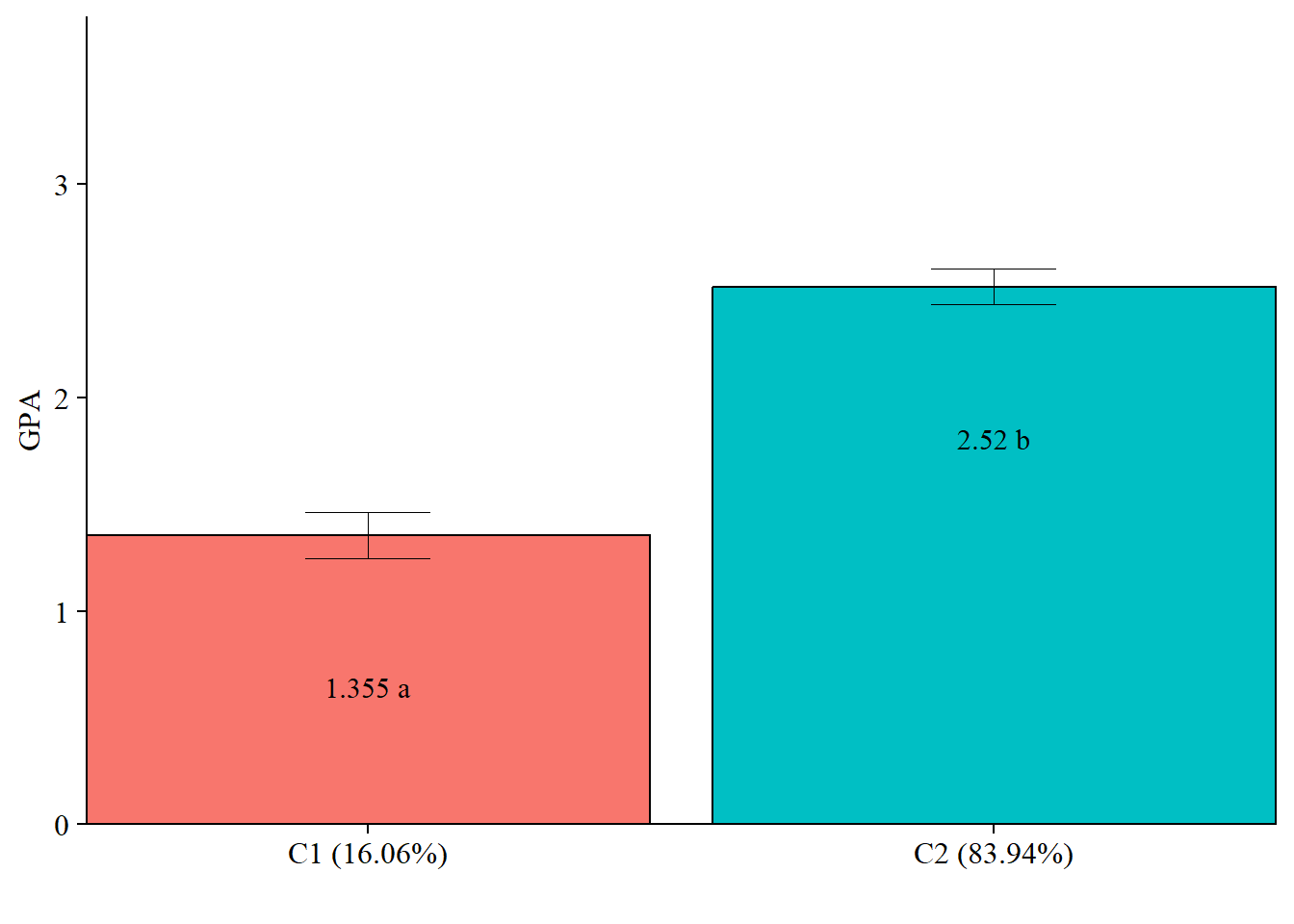
                            check=TRUE, run = TRUE, hashfilename = FALSE)

---

14.4.1.2 Plot Distal Outcome mean differences

modelParams <- readModels(here("three_step", "auto_3step", "c2_du3step.out"))

# Extract class size 
c_size <- as.data.frame(modelParams[["class_counts"]][["modelEstimated"]][["proportion"]]) %>% 
  rename("cs" = 1) %>% 
  mutate(cs = round(cs*100, 2))

c_size_val <- paste0("C", 1:nrow(c_size), glue(" ({c_size[1:nrow(c_size),]}%)"))


# Extract information as data frame
estimates <- as.data.frame(modelParams[["lcCondMeans"]][["overall"]]) %>%
  reshape2::melt(id.vars = "var") %>%
  mutate(variable = as.character(variable),
         LatentClass = case_when(
           endsWith(variable, "1") ~ c_size_val[1],
           endsWith(variable, "2") ~ c_size_val[2])) %>% #Add to this based on the number of classes you have
  head(-3) %>% 
  pivot_wider(names_from = variable, values_from = value) %>% 
  unite("mean", contains("m"), na.rm = TRUE) %>% 
  unite("se", contains("se"), na.rm = TRUE) %>% 
  mutate(across(c(mean, se), as.numeric))

# Add labels (NOTE: You must change the labels to match the significance testing!!) 
value_labels <- paste0(estimates$mean, c(" a"," b"))

# Plot bar graphs
estimates %>%
  ggplot(aes(fill = LatentClass, y = mean, x = LatentClass)) +
  geom_bar(position = "dodge", stat = "identity", color = "black") +
  geom_errorbar(aes(ymin=mean-se, ymax=mean+se),
                size=.3,    
                width=.2,
                position=position_dodge(.9)) +
  geom_text(aes(y = mean, label = value_labels), 
            family = "serif", size = 4,
            position=position_dodge(.9),
            vjust = 8) +
  #scale_fill_grey(start = .5, end = .7) +
  labs(y="GPA", x="") +
  theme_cowplot() +
  theme(text = element_text(family = "serif", size = 12),
        axis.text.x = element_text(size=12),
        legend.position="none") +
  coord_cartesian(expand = FALSE, 
                  ylim=c(0,max(estimates$mean*1.5))) # Change ylim based on distal outcome rang

# Save plot
ggsave(here("figures","Du3STEP_plot.jpeg"),                
       dpi=300, width=10, height = 7, units="in")