20 Adding Covariates
Data Source: The data used to illustrate these analyses include elementary school student Science Attitude survey items collected during 7th and 10th grades from the Longitudinal Study of American Youth (LSAY; Miller, 2015).
To install package {rhdf5}
if (!requireNamespace("BiocManager", quietly = TRUE))
  install.packages("BiocManager")

#BiocManager::install("rhdf5")
Load packages
library(MplusAutomation)
library(rhdf5)
library(tidyverse)
library(here)
library(glue)
library(janitor)
library(gt)
library(reshape2)
library(cowplot)
library(ggrepel)
library(haven)
library(modelsummary)
library(corrplot)
library(DiagrammeR)
library(filesstrings)
library(PNWColors)
Read in LSAY data file, lsay_new.csv.
lsay_data <- read_csv(here("data","lsay_lta.csv"), na = c("9999")) %>%
    mutate(across(everything(), as.numeric))
20.1 Descriptive Statistics
20.1.1 Data Summary
data <- lsay_data

select_data <- data %>%
 select(female, minority, ab39m:ga33l)

f <- All(select_data) ~ Mean + SD + Min + Median + Max + Histogram
datasummary(f, data, output="markdown")| Mean | SD | Min | Median | Max | Histogram | |
|---|---|---|---|---|---|---|
| female | 0.48 | 0.50 | 0.00 | 0.00 | 1.00 | ▇▆ |
| minority | 0.23 | 0.42 | 0.00 | 0.00 | 1.00 | ▇▂ |
| ab39m | 0.61 | 0.49 | 0.00 | 1.00 | 1.00 | ▄▇ |
| ab39t | 0.40 | 0.49 | 0.00 | 0.00 | 1.00 | ▇▅ |
| ab39u | 0.49 | 0.50 | 0.00 | 0.00 | 1.00 | ▇▇ |
| ab39w | 0.40 | 0.49 | 0.00 | 0.00 | 1.00 | ▇▅ |
| ab39x | 0.46 | 0.50 | 0.00 | 0.00 | 1.00 | ▇▆ |
| ga33a | 0.58 | 0.49 | 0.00 | 1.00 | 1.00 | ▅▇ |
| ga33h | 0.43 | 0.49 | 0.00 | 0.00 | 1.00 | ▇▅ |
| ga33i | 0.51 | 0.50 | 0.00 | 1.00 | 1.00 | ▇▇ |
| ga33k | 0.42 | 0.49 | 0.00 | 0.00 | 1.00 | ▇▅ |
| ga33l | 0.42 | 0.49 | 0.00 | 0.00 | 1.00 | ▇▅ |
20.2 Adding Covariates
Continuing from the previous section 18, we use the ML three-step method to estimate LTA models with predictors and distal outcomes). Estimate the unconditional model for each latent variable with the predictors included in the auxiliary option for at least one of the models.
Covariates
-
sci_issues7: Interest in science issues (1 = Not at all interested, 2 = Moderately Interested, 3 = Very interested)
-
sci_irt7: 7th Grade Science IRT Score (Continuous)
-
female: Gender (0 = Male, 1 = Female)
20.2.1 Step 1 - Estimate Unconditional Model w/ Auxiliary Specification
7th Grade
step1  <- mplusObject(
  TITLE = "Step 1 - T1",
  VARIABLE =
  "usevar = ab39m ab39t ab39u ab39w ab39x;
  categorical = ab39m ab39t ab39u ab39w ab39x;

   classes = c(4);

   auxiliary = sci_issues7 sci_irt7 female;

   idvariable = casenum;",

  ANALYSIS =
   "estimator = mlr;
    type = mixture;
    starts = 0;
    optseed = 534483;",

  SAVEDATA =
   "File=3step_t1.dat;
    Save=cprob;",

  OUTPUT = "residual tech11 tech14 svalues",

  PLOT =
    "type = plot3;
    series = ab39m-ab39x(*);",

  usevariables = colnames(lsay_data),
  rdata = lsay_data)

step1_fit <- mplusModeler(step1,
                            dataout=here("lta","cov_model","t1.dat"),
                            modelout=here("lta","cov_model","one_T1.inp") ,
                            check=TRUE, run = TRUE, hashfilename = FALSE)
10th Grade
step1  <- mplusObject(
  TITLE = "Step 1 - T1",
  VARIABLE =
  "usevar =  ga33a ga33h ga33i ga33k ga33l;
  categorical =  ga33a ga33h ga33i ga33k ga33l;

   classes = c(4);

   !auxiliary = sci_issues7 sci_irt7 female;

   idvariable = casenum;",

  ANALYSIS =
   "estimator = mlr;
    type = mixture;
    starts = 0;
    optseed = 392418;",

  SAVEDATA =
   "File=3step_t2.dat;
    Save=cprob;",

  OUTPUT = "residual tech11 tech14 svalues",

  PLOT =
    "type = plot3;
    series = ga33a-ga33l(*);",

  usevariables = colnames(lsay_data),
  rdata = lsay_data)

step1_fit <- mplusModeler(step1,
                            dataout=here("lta","cov_model","t2.dat"),
                            modelout=here("lta","cov_model","one_T2.inp") ,
                            check=TRUE, run = TRUE, hashfilename = FALSE)
plot_lca_function requires 5 arguments:
-
model_name: name of Mplus model object (e.g.,model_t1_c4) -
item_num: the number of items in LCA measurement model (e.g.,5) -
class_num: the number of classes (k) in LCA model (e.g.,4) -
item_labels: the item labels for x-axis (e.g.,c("Enjoy","Useful","Logical","Job","Adult")) -
plot_title: include the title of the plot here (e.g.,"Time 1 LCA Conditional Item Probability Plot")
plot_lca_function <- function(model_name,item_num,class_num,item_labels,plot_title){
mplus_model <- as.data.frame(model_name$gh5$means_and_variances_data$estimated_probs$values)
plot_t1 <- mplus_model[seq(2, 2*item_num, 2),]
c_size <- as.data.frame(model_name$class_counts$modelEstimated$proportion)
colnames(c_size) <- paste0("cs")
c_size <- c_size %>% mutate(cs = round(cs*100, 2))
colnames(plot_t1) <- paste0("C", 1:class_num, glue(" ({c_size[1:class_num,]}%)"))
plot_t1 <- cbind(Var = paste0("U", 1:item_num), plot_t1)
plot_t1$Var <- factor(plot_t1$Var,
labels = item_labels)
plot_t1$Var <- fct_inorder(plot_t1$Var)
pd_long_t1 <- melt(plot_t1, id.vars = "Var")
p <- pd_long_t1 %>%
ggplot(aes(x = as.integer(Var), y = value,
shape = variable, colour = variable, lty = variable)) +
geom_point(size = 4) + geom_line() +
scale_x_continuous("", breaks = 1:5, labels = plot_t1$Var) +
scale_colour_grey() +
labs(title = plot_title, y = "Probability") +
theme_cowplot() +
theme(legend.title = element_blank(),
legend.position = "top")
p
return(p)
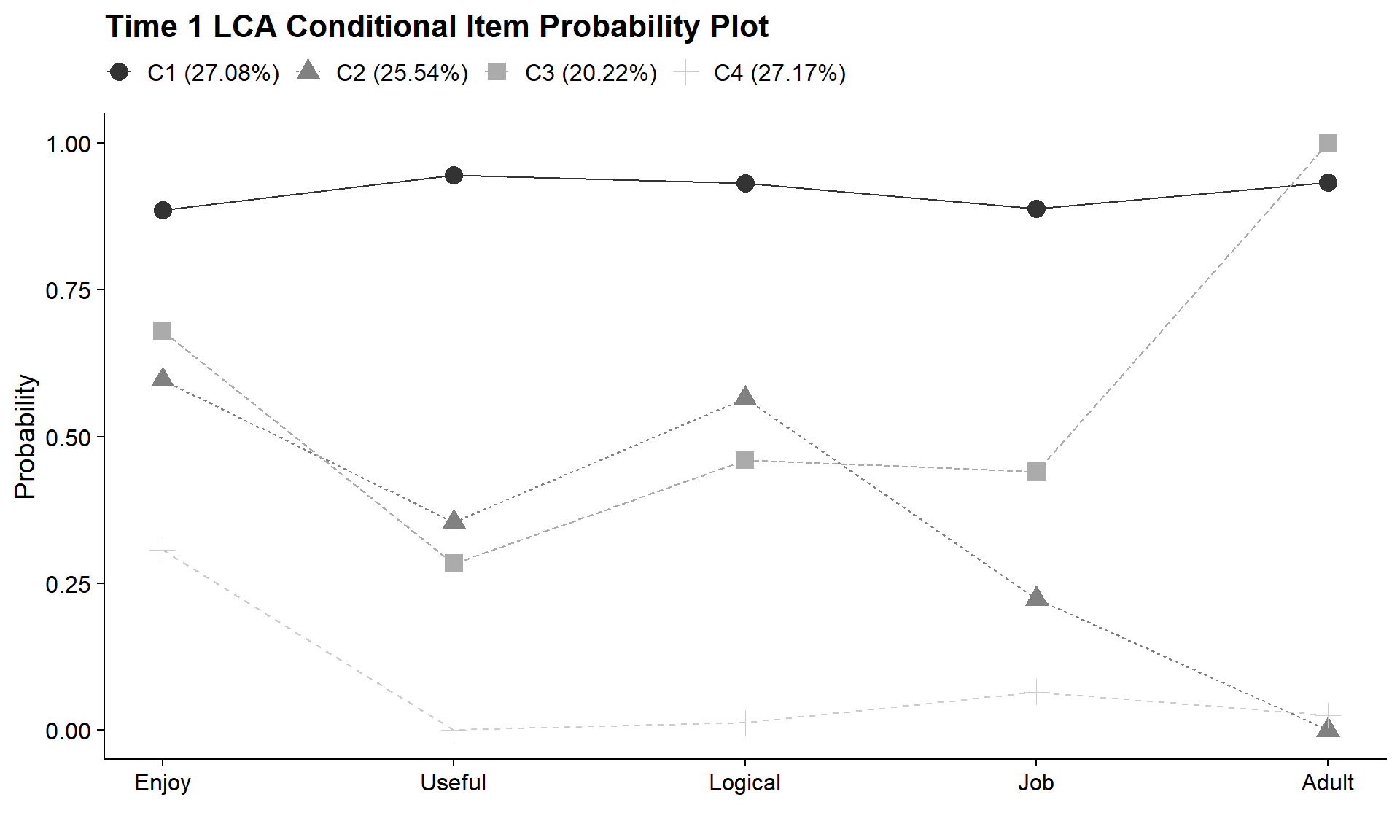
}Plot Time 1
output_T1 <- readModels(here("lta","cov_model","one_T1.out"))

plot_lca_function(
  model_name = output_T1,
  item_num = 5,
  class_num = 4,
  item_labels = c("Enjoy","Useful","Logical","Job","Adult"),
  plot_title = "Time 1 LCA Conditional Item Probability Plot"
  )
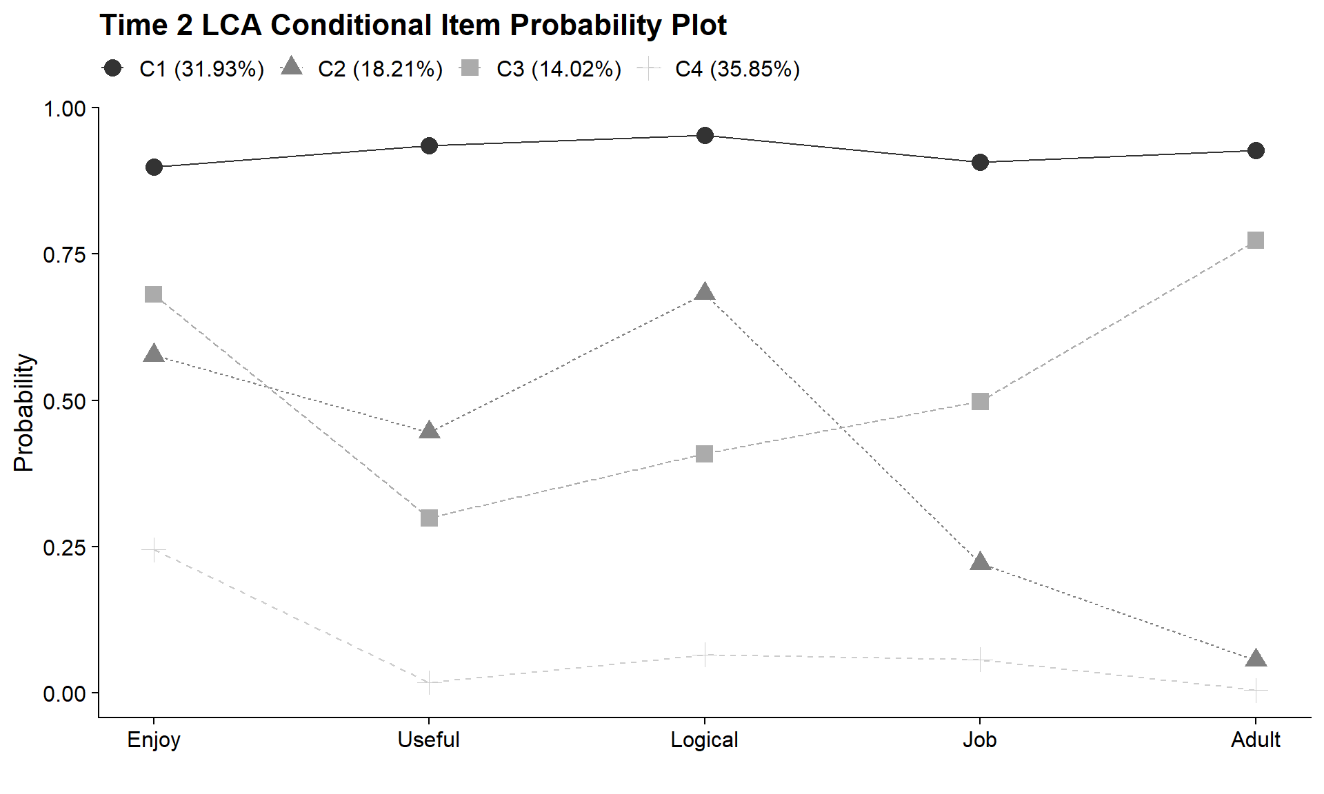
Plot Time 2
output_T2 <- readModels(here("lta","cov_model","one_T2.out"))

plot_lca_function(
  model_name = output_T2,
  item_num = 5,
  class_num = 4,
  item_labels = c("Enjoy","Useful","Logical","Job","Adult"),
  plot_title = "Time 2 LCA Conditional Item Probability Plot"
  )
20.2.2 Step 2 - Determine Measurement Error
Extract logits for the classification probabilities for the most likely latent class:
logit_cprobs_T1 <- as.data.frame(output_T1[["class_counts"]]
                                       [["logitProbs.mostLikely"]])

logit_cprobs_T2 <- as.data.frame(output_T2[["class_counts"]]
                                       [["logitProbs.mostLikely"]])
Extract saved dataset:
savedata_T1 <- as.data.frame(output_T1[["savedata"]])
savedata_T2 <- as.data.frame(output_T2[["savedata"]])
Rename the column in savedata named “C” and change to “N”
colnames(savedata_T1)[colnames(savedata_T1)=="C"] <- "N_T1"
colnames(savedata_T2)[colnames(savedata_T2)=="C"] <- "N_T2"

savedata <- savedata_T1 %>%
  full_join(savedata_T2, by = "CASENUM")
20.2.3 Step 3 - Add Auxiliary Variables
Here, we add covariates and distal outcomes to the overall model statement. This specifies the overall relationship between observed covariates and the latent classes at cross sectional timepoints.
step3  <- mplusObject(
  TITLE = "ML Three Step LTA Model",

  VARIABLE =
 "nominal=N_T1 N_T2;
  usevar = N_T1 N_T2 SCI_IRT7 FEMALE;
  classes = c1(4) c2(4);" ,

  ANALYSIS =
 "estimator = mlr;
  type = mixture;
  starts = 0;",

  MODEL =
  glue(
 " %OVERALL%

   c2 on c1;
   c1 c2 on  SCI_IRT7 FEMALE;

  MODEL c1:

  %c1#1%
  [N_T1#1@{logit_cprobs_T1[1,1]}];
  [N_T1#2@{logit_cprobs_T1[1,2]}];
  [N_T1#3@{logit_cprobs_T1[1,3]}];

  %c1#2%
  [N_T1#1@{logit_cprobs_T1[2,1]}];
  [N_T1#2@{logit_cprobs_T1[2,2]}];
  [N_T1#3@{logit_cprobs_T1[2,3]}];

  %c1#3%
  [N_T1#1@{logit_cprobs_T1[3,1]}];
  [N_T1#2@{logit_cprobs_T1[3,2]}];
  [N_T1#3@{logit_cprobs_T1[3,3]}];

  %c1#4%
  [N_T1#1@{logit_cprobs_T1[4,1]}];
  [N_T1#2@{logit_cprobs_T1[4,2]}];
  [N_T1#3@{logit_cprobs_T1[4,3]}];


  MODEL c2:

  %c2#1%
  [N_T2#1@{logit_cprobs_T2[1,1]}];
  [N_T2#2@{logit_cprobs_T2[1,2]}];
  [N_T2#3@{logit_cprobs_T2[1,3]}];

  %c2#2%
  [N_T2#1@{logit_cprobs_T2[2,1]}];
  [N_T2#2@{logit_cprobs_T2[2,2]}];
  [N_T2#3@{logit_cprobs_T2[2,3]}];


  %c2#3%
  [N_T2#1@{logit_cprobs_T2[3,1]}];
  [N_T2#2@{logit_cprobs_T2[3,2]}];
  [N_T2#3@{logit_cprobs_T2[3,3]}];

   %c2#4%
  [N_T2#1@{logit_cprobs_T2[4,1]}];
  [N_T2#2@{logit_cprobs_T2[4,2]}];
  [N_T2#3@{logit_cprobs_T2[4,3]}];"),


  OUTPUT = "tech15;",

  usevariables = colnames(savedata),
  rdata = savedata)

step3_fit <- mplusModeler(step3,
               dataout=here("lta","cov_model","three.dat"),
               modelout=here("lta","cov_model","three.inp"),
               check=TRUE, run = TRUE, hashfilename = FALSE)
20.2.3.1 LTA Transition Plot
This code is adapted from the source code for the plotLTA function found in the
NOTE: The function found in plot_transitions_function.R is specific to a model with 2 time-points and 4-classes & must be updated to accommodate other models.
source(here("functions","plot_transitions_function.R"))

lta_model <- readModels(here("lta","cov_model","three.out"))

plot_transitions_function(
  model_name = lta_model,
  color_pallete = pnw_palette("Bay", n=4, type = "discrete"),
  facet_labels =c(
    `1` = "Transitions to 10th Grade from the Pro-Science w/ Elevated Utility Class",
    `2` = "Transitions to 10th Grade from the Ambivalent w/ Elevated Utility Class",
    `3` = "Transitions to 10th Grade from the Ambivalent w/ Minimal Utility Class",
    `4` = "Transitions to 10th Grade from the Anti-Science w/ Minimal Utility Class"),
  timepoint_labels = c('1' = "7th Grade", '2' = "10th Grade"),
  class_labels = c(
    "Pro-Science",
    "Amb. / Elev. Utility",
    "Amb. / Min. Utility",
    "Anti-Science")
  )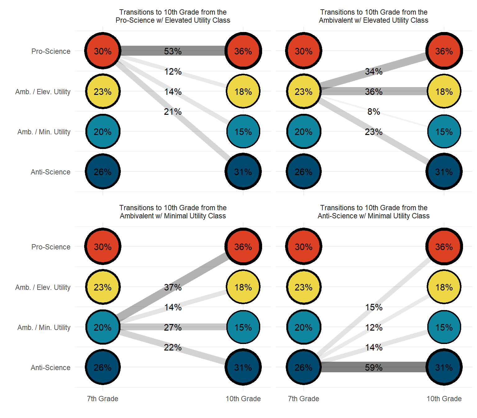
Table:
Transition probability across classes can also be described using a table, or transition matrix. The table shows the 7th grade classes by 10th grade latent class, with the cells represented the overall transition.
lta_prob <- as.data.frame(lta_model$class_counts$transitionProbs$probability)


t_matrix <- tibble(
  "7th Grade" = c("Pro-Science","Amb. / Elev. Utility","Amb. / Min. Utility","Anti-Science"),
  "Pro-Science" = c(lta_prob[1,1],lta_prob[2,1],lta_prob[3,1],lta_prob[4,1]),
  "Amb. / Elev. Utility" = c(lta_prob[5,1],lta_prob[6,1],lta_prob[7,1],lta_prob[8,1]),
  "Amb. / Min. Utility" = c(lta_prob[9,1],lta_prob[10,1],lta_prob[11,1],lta_prob[12,1]),
  "Anti-Science" = c(lta_prob[13,1],lta_prob[14,1],lta_prob[15,1],lta_prob[16,1]))

t_matrix %>%
  gt(rowname_col = "7th Grade") %>%
  tab_stubhead(label = "7th Grade") %>%
  tab_header(
    title = md("**Transition Probabilities**")) %>%
  fmt_number(2:5,decimals = 2) %>%
tab_spanner(label = "10th Grade",columns = 2:5)#%>% | Transition Probabilities | ||||
| 7th Grade |
10th Grade
|
|||
|---|---|---|---|---|
| Pro-Science | Amb. / Elev. Utility | Amb. / Min. Utility | Anti-Science | |
| Pro-Science | 0.53 | 0.12 | 0.14 | 0.21 |
| Amb. / Elev. Utility | 0.34 | 0.35 | 0.08 | 0.23 |
| Amb. / Min. Utility | 0.37 | 0.14 | 0.27 | 0.22 |
| Anti-Science | 0.15 | 0.12 | 0.14 | 0.59 |
#gtsave("matrix.docx")20.2.3.2 Covariate Table
The covariate table shows the relationship between covariate (gender) and distal outcome (IRT score) and latent classes for both cross sectional timepoints.
# REFERENCE CLASS 4
cov <- as.data.frame(lta_model[["parameters"]][["unstandardized"]]) %>%
  filter(param %in% c("SCI_IRT7", "FEMALE")) %>%
  mutate(param = case_when(
            param == "SCI_IRT7" ~ "Science IRT Score",
            param == "FEMALE" ~ "Gender"),
    se = paste0("(", format(round(se,2), nsmall =2), ")")) %>%
  separate(paramHeader, into = c("Time", "Class"), sep = "#") %>%
  mutate(Class = case_when(
            Class == "1.ON" ~ "Pro-Science",
            Class == "2.ON" ~ "Amb. / Elev. Utility",
            Class == "3.ON" ~ "Amb. / Min. Utility"),
         Time = case_when(
            Time == "C1" ~ "7th Grade (T1)",
            Time == "C2" ~ "10th Grade (T2)",
         )
         ) %>%
  unite(estimate, est, se, sep = " ") %>%
  select(Time:pval, -est_se) %>%
  mutate(pval = ifelse(pval<0.001, paste0("<.001*"),
                       ifelse(pval<0.05, paste0(scales::number(pval, accuracy = .001), "*"),
                              scales::number(pval, accuracy = .001))))


# Create table

cov_m1 <- cov %>%
  group_by(param, Class) %>%
  gt() %>%
  tab_header(
    title = "Relations Between the Covariates and Latent Class") %>%
  tab_footnote(
    footnote = md(
      "Reference Group: Anti-Science"
    ),
locations = cells_title()
  ) %>%
  cols_label(
    param = md("Covariate"),
    estimate = md("Estimate (*se*)"),
    pval = md("*p*-value")) %>%
  sub_missing(1:3,
              missing_text = "") %>%
  sub_values(values = c(999.000), replacement = "-") %>%
  cols_align(align = "center") %>%
  opt_align_table_header(align = "left") %>%
  gt::tab_options(table.font.names = "serif")

cov_m1| Relations Between the Covariates and Latent Class1 | ||
| Time | Estimate (se) | p-value |
|---|---|---|
| Science IRT Score - Pro-Science | ||
| 7th Grade (T1) | 0.05 (0.01) | <.001* |
| 10th Grade (T2) | 0.056 (0.01) | <.001* |
| Gender - Pro-Science | ||
| 7th Grade (T1) | -1.001 (0.23) | <.001* |
| 10th Grade (T2) | 0.011 (0.22) | 0.962 |
| Science IRT Score - Amb. / Elev. Utility | ||
| 7th Grade (T1) | -0.012 (0.01) | 0.351 |
| 10th Grade (T2) | 0.049 (0.02) | 0.002* |
| Gender - Amb. / Elev. Utility | ||
| 7th Grade (T1) | -0.515 (0.28) | 0.071 |
| 10th Grade (T2) | -0.111 (0.33) | 0.737 |
| Science IRT Score - Amb. / Min. Utility | ||
| 7th Grade (T1) | 0.021 (0.01) | 0.093 |
| 10th Grade (T2) | 0.022 (0.02) | 0.202 |
| Gender - Amb. / Min. Utility | ||
| 7th Grade (T1) | -0.761 (0.26) | 0.003* |
| 10th Grade (T2) | 0.075 (0.32) | 0.815 |
| 1 Reference Group: Anti-Science | ||
20.2.3.3 Manually calculate transition probabilities by covariate
Optionally, transition probabilities can be calculated for each level of the covariate. For example, transition probabilities for males or females only, depending on the research question.
step3  <- mplusObject(
  TITLE = "LTA (invariant)",

  VARIABLE =
 "usevar = ab39m ab39t ab39u ab39w ab39x  ! 7th grade indicators
               ga33a ga33h ga33i ga33k ga33l FEMALE;
  categorical = ab39m-ab39x ga33a-ga33l;
  classes = c1(4) c2(4);" ,

  ANALYSIS =
 "estimator = mlr;
  type = mixture;
  starts = 500 100;
 processors = 10;",

  MODEL =
  "%overall%

    c2 c1 on FEMALE;

      c2#1 on c1#1 (b11);
      c2#2 on c1#1 (b21);
      c2#3 on c1#1 (b31);

      c2#1 on c1#2 (b12);
      c2#2 on c1#2 (b22);
      c2#3 on c1#2 (b32);

      c2#1 on c1#3 (b13);
      c2#2 on c1#3 (b23);
      c2#3 on c1#3 (b33);

      [c2#1] (a1);
      [c2#2] (a2);
      [c2#3] (a3);

     c2#1 ON female (b212);
     c2#2 ON female (b222);
     c2#3 ON female (b232);
     c1#1 ON female (b112);
     c1#2 ON female (b122);
     c1#3 ON female (b132);

      MODEL c1:
      %c1#1%
      [AB39M$1-AB39X$1] (1-5);  !!! labels that are repeated will constrain parameters to equality !!!
      %c1#2%
      [AB39M$1-AB39X$1] (6-10);
      %c1#3%
      [AB39M$1-AB39X$1] (11-15);
      %c1#4%
      [AB39M$1-AB39X$1] (16-20);

      MODEL c2:
      %c2#1%
      [GA33A$1-GA33L$1] (1-5);
      %c2#2%
      [GA33A$1-GA33L$1] (6-10);
      %c2#3%
      [GA33A$1-GA33L$1] (11-15);
      %c2#4%
      [GA33A$1-GA33L$1] (16-20);",


  OUTPUT = "tech1 tech15 svalues;",

  MODELCONSTRAINT = "  ! Compute joint and marginal probabilities:
        New(
        t11 t12 t13 t14
        t21 t22 t23 t24
        t31 t32 t33 t34
        t41 t42 t43 t44

        t11B t12B t13B t14B
        t21B t22B t23B t24B
        t31B t32B t33B t34B
        t41B t42B t43B t44B

        diff_11_22 x

       );

        t11 = exp(a1 +b11)/(exp(a1+b11)+exp(a2+b21)+exp(a3+b31)+exp(0));
        t12 = exp(a2 +b21)/(exp(a1+b11)+exp(a2+b21)+exp(a3+b31)+exp(0));
        t13 = exp(a3 +b31)/(exp(a1+b11)+exp(a2+b21)+exp(a3+b31)+exp(0));
        t14 = 1 - (t11+t12+t13);

        t21 = exp(a1 +b12)/(exp(a1+b12)+exp(a2+b22)+exp(a3+b32)+exp(0));
        t22 = exp(a2 +b22)/(exp(a1+b12)+exp(a2+b22)+exp(a3+b32)+exp(0));
        t23 = exp(a3 +b32)/(exp(a1+b12)+exp(a2+b22)+exp(a3+b32)+exp(0));
        t24 = 1 - (t21+t22+t23);

        t31 = exp(a1 +b13)/(exp(a1+b13)+exp(a2+b23)+exp(a3+b33)+exp(0));
        t32 = exp(a2 +b23)/(exp(a1+b13)+exp(a2+b23)+exp(a3+b33)+exp(0));
        t33 = exp(a3 +b33)/(exp(a1+b13)+exp(a2+b23)+exp(a3+b33)+exp(0));
        t34 = 1 - (t31+t32+t33);

        t41 = exp(a1)/(exp(a1)+exp(a2)+exp(a3)+exp(0));
        t42 = exp(a2)/(exp(a1)+exp(a2)+exp(a3)+exp(0));
        t43 = exp(a3)/(exp(a1)+exp(a2)+exp(a3)+exp(0));
        t44 = 1 - (t41+t42+t43);


     !c1#3 ON female (b132);

 x= 1  ; ! x=1 is female, x=0 males

t11B = exp(a1 +b11+b212*x)/(exp(a1+b11+b212*x)+exp(a2+b21+b222*x)+exp(a3+b31+b232*x)
+exp(0));
t12B = exp(a2 +b21+b222*x)/(exp(a1+b11+b212*x)+exp(a2+b21+b222*x)+exp(a3+b31+b232*x)
+exp(0));
t13B = exp(a3 +b31+b232*x)/(exp(a1+b11+b212*x)+exp(a2+b21+b222*x)+exp(a3+b31+b232*x)
+exp(0));
t14B = 1 - (t11B+t12B+t13B);

t21B = exp(a1 +b12+b212*x)/(exp(a1+b12+b212*x)+exp(a2+b22+b222*x)+exp(a3+b32+b232*x)
+exp(0));
t22B = exp(a2 +b22+b222*x)/(exp(a1+b12+b212*x)+exp(a2+b22+b222*x)+exp(a3+b32+b232*x)
+exp(0));
t23B = exp(a3 +b32+b232*x)/(exp(a1+b12+b212*x)+exp(a2+b22+b222*x)+exp(a3+b32+b232*x)
+exp(0));
t24B = 1 - (t21B+t22B+t23B);

t31B = exp(a1 +b13+b212*x)/(exp(a1+b13+b212*x)+exp(a2+b23+b222*x)+exp(a3+b33+b232*x)
+exp(0));
t32B = exp(a2 +b23+b222*x)/(exp(a1+b13+b212*x)+exp(a2+b23+b222*x)+exp(a3+b33+b232*x)
+exp(0));
t33B = exp(a3 +b33+b232*x)/(exp(a1+b13+b212*x)+exp(a2+b23+b222*x)+exp(a3+b33+b232*x)
+exp(0));
t34B = 1 - (t31B+t32B+t33B);

t41B = exp(a1+b212*x)/(exp(a1+b212*x)+exp(a2+b222*x)+exp(a3+b232*x)+exp(0));
t42B = exp(a2+b222*x)/(exp(a1+b212*x)+exp(a2+b222*x)+exp(a3+b232*x)+exp(0));
t43B = exp(a3+b232*x)/(exp(a1+b212*x)+exp(a2+b222*x)+exp(a3+b232*x)+exp(0));
t44B = 1 - (t41B+t42B+t43B);

        diff_11_22= t11-t11B;",

  usevariables = colnames(savedata),
  rdata = savedata)

step3_fit <- mplusModeler(step3,
               dataout=here("lta","cov_model","calc_tran.dat"),
               modelout=here("lta","cov_model","calc_tran.inp"),
               check=TRUE, run = TRUE, hashfilename = FALSE)
Read invariance model and extract parameters (intercepts and multinomial regression coefficients)
lta_inv1 <- readModels(here("lta","cov_model","calc_tran.out" ), quiet = TRUE)

par <- as_tibble(lta_inv1[["parameters"]][["unstandardized"]]) %>%
  select(1:3) %>%
  filter(grepl('ON|Means|Intercept', paramHeader)) %>%
  mutate(est = as.numeric(est),
         label = c("b11", "b12", "b13", "b21", "b22", "b23", "b31", "b32", "b33", "b212", "b222", "b232", "b112", "b122", "b132", "a11", "a21", "a31", "a12", "a22", "a32"))
Manual method to calculate transition probabilities by covariate:
# Name each parameter individually to make the subsequent calculations more readable
a1 <- unlist(par[19,3]);
a2 <- unlist(par[20,3]);
a3 <- unlist(par[21,3]);

b11 <- unlist(par[1,3]);
b21 <- unlist(par[4,3]);
b31 <- unlist(par[7,3]);

b12 <- unlist(par[2,3]);
b22 <- unlist(par[5,3]);
b32 <- unlist(par[8,3]);

b13 <- unlist(par[3,3]);
b23 <- unlist(par[6,3]);
b33 <- unlist(par[9,3]);

b212 <- unlist(par[10,3]);
b222 <- unlist(par[11,3]);
b232 <- unlist(par[12,3]);

b112 <- unlist(par[13,3]);
b122 <- unlist(par[14,3]);
b132 <- unlist(par[15,3]);

x <- 0 # x=1 is female, x=0 males

# Calculate transition probabilities from the logit parameters
t11B <- exp(a1 + b11 + b212*x) / (exp(a1 + b11 + b212*x) + exp(a2 + b21 + b222*x) + exp(a3 + b31 + b232*x) + exp(0))
t12B <- exp(a2 + b21 + b222*x) / (exp(a1 + b11 + b212*x) + exp(a2 + b21 + b222*x) + exp(a3 + b31 + b232*x) + exp(0))
t13B <- exp(a3 + b31 + b232*x) / (exp(a1 + b11 + b212*x) + exp(a2 + b21 + b222*x) + exp(a3 + b31 + b232*x) + exp(0))
t14B <- 1 - (t11B + t12B + t13B)

t21B <- exp(a1 + b12 + b212*x) / (exp(a1 + b12 + b212*x) + exp(a2 + b22 + b222*x) + exp(a3 + b32 + b232*x) + exp(0))
t22B <- exp(a2 + b22 + b222*x) / (exp(a1 + b12 + b212*x) + exp(a2 + b22 + b222*x) + exp(a3 + b32 + b232*x) + exp(0))
t23B <- exp(a3 + b32 + b232*x) / (exp(a1 + b12 + b212*x) + exp(a2 + b22 + b222*x) + exp(a3 + b32 + b232*x) + exp(0))
t24B <- 1 - (t21B + t22B + t23B)

t31B <- exp(a1 + b13 + b212*x) / (exp(a1 + b13 + b212*x) + exp(a2 + b23 + b222*x) + exp(a3 + b33 + b232*x) + exp(0))
t32B <- exp(a2 + b23 + b222*x) / (exp(a1 + b13 + b212*x) + exp(a2 + b23 + b222*x) + exp(a3 + b33 + b232*x) + exp(0))
t33B <- exp(a3 + b33 + b232*x) / (exp(a1 + b13 + b212*x) + exp(a2 + b23 + b222*x) + exp(a3 + b33 + b232*x) + exp(0))
t34B <- 1 - (t31B + t32B + t33B)

t41B <- exp(a1 + b212*x) / (exp(a1 + b212*x) + exp(a2 + b222*x) + exp(a3 + b232*x) + exp(0))
t42B <- exp(a2 + b222*x) / (exp(a1 + b212*x) + exp(a2 + b222*x) + exp(a3 + b232*x) + exp(0))
t43B <- exp(a3 + b232*x) / (exp(a1 + b212*x) + exp(a2 + b222*x) + exp(a3 + b232*x) + exp(0))
t44B <- 1 - (t41B + t42B + t43B)

x <- 1 # x=1 is female, x=0 males

# Calculate transition probabilities from the logit parameters
t11 <- exp(a1 + b11 + b212*x) / (exp(a1 + b11 + b212*x) + exp(a2 + b21 + b222*x) + exp(a3 + b31 + b232*x) + exp(0))
t12 <- exp(a2 + b21 + b222*x) / (exp(a1 + b11 + b212*x) + exp(a2 + b21 + b222*x) + exp(a3 + b31 + b232*x) + exp(0))
t13 <- exp(a3 + b31 + b232*x) / (exp(a1 + b11 + b212*x) + exp(a2 + b21 + b222*x) + exp(a3 + b31 + b232*x) + exp(0))
t14 <- 1 - (t11 + t12 + t13)

t21 <- exp(a1 + b12 + b212*x) / (exp(a1 + b12 + b212*x) + exp(a2 + b22 + b222*x) + exp(a3 + b32 + b232*x) + exp(0))
t22 <- exp(a2 + b22 + b222*x) / (exp(a1 + b12 + b212*x) + exp(a2 + b22 + b222*x) + exp(a3 + b32 + b232*x) + exp(0))
t23 <- exp(a3 + b32 + b232*x) / (exp(a1 + b12 + b212*x) + exp(a2 + b22 + b222*x) + exp(a3 + b32 + b232*x) + exp(0))
t24 <- 1 - (t21 + t22 + t23)

t31 <- exp(a1 + b13 + b212*x) / (exp(a1 + b13 + b212*x) + exp(a2 + b23 + b222*x) + exp(a3 + b33 + b232*x) + exp(0))
t32 <- exp(a2 + b23 + b222*x) / (exp(a1 + b13 + b212*x) + exp(a2 + b23 + b222*x) + exp(a3 + b33 + b232*x) + exp(0))
t33 <- exp(a3 + b33 + b232*x) / (exp(a1 + b13 + b212*x) + exp(a2 + b23 + b222*x) + exp(a3 + b33 + b232*x) + exp(0))
t34 <- 1 - (t31 + t32 + t33)

t41 <- exp(a1 + b212*x) / (exp(a1 + b212*x) + exp(a2 + b222*x) + exp(a3 + b232*x) + exp(0))
t42 <- exp(a2 + b222*x) / (exp(a1 + b212*x) + exp(a2 + b222*x) + exp(a3 + b232*x) + exp(0))
t43 <- exp(a3 + b232*x) / (exp(a1 + b212*x) + exp(a2 + b222*x) + exp(a3 + b232*x) + exp(0))
t44 <- 1 - (t41 + t42 + t43)
Create table
20.2.4 Create Transition Table
The table below shows the transition probabilities estimated for girls only. These are hand calculated in Mplus using the OVERALL section of the model and Model Constraints command.
t_matrix <- tibble(
  "Time1" = c("C1=Anti-Science","C1=Amb. w/ Elevated","C1=Amb. w/ Minimal","C1=Pro-Science"),
  "C2=Anti-Science" = c(t11,t21,t31,t41),
  "C2=Amb. w/ Elevated" = c(t12,t22,t32,t42),
  "C2=Amb. w/ Minimal" = c(t13,t23,t33,t43),
  "C2=Pro-Science" = c(t14,t24,t34,t44))

t_matrix %>%
  gt(rowname_col = "Time1") %>%
  tab_stubhead(label = "7th grade") %>%
  tab_header(
    title = md("**FEMALES: Student transitions from 7th grade (rows) to 10th grade (columns)**")) %>%
  fmt_number(2:5,decimals = 3) %>%
  tab_spanner(label = "10th grade",columns = 2:5) %>%
  tab_footnote(
    footnote = md(
    "*Note.* Transition matrix values are the identical to Table 5, however Table 5
    has the values rearranged by class for interpretation purposes. Classes may be arranged
    directly through Mplus syntax using start values."),
locations = cells_title())| FEMALES: Student transitions from 7th grade (rows) to 10th grade (columns)1 | ||||
| 7th grade |
10th grade
|
|||
|---|---|---|---|---|
| C2=Anti-Science | C2=Amb. w/ Elevated | C2=Amb. w/ Minimal | C2=Pro-Science | |
| C1=Anti-Science | 0.302 | 0.261 | 0.097 | 0.341 |
| C1=Amb. w/ Elevated | 0.129 | 0.510 | 0.152 | 0.209 |
| C1=Amb. w/ Minimal | 0.164 | 0.308 | 0.273 | 0.255 |
| C1=Pro-Science | 0.177 | 0.187 | 0.094 | 0.542 |
| 1 Note. Transition matrix values are the identical to Table 5, however Table 5 has the values rearranged by class for interpretation purposes. Classes may be arranged directly through Mplus syntax using start values. | ||||
t_matrix <- tibble(
  "Time1" = c("C1=Anti-Science","C1=Amb. w/ Elevated","C1=Amb. w/ Minimal","C1=Pro-Science"),
  "C2=Anti-Science" = c(t11B,t21B,t31B,t41B),
  "C2=Amb. w/ Elevated" = c(t12B,t22B,t32B,t42B),
  "C2=Amb. w/ Minimal" = c(t13B,t23B,t33B,t43B),
  "C2=Pro-Science" = c(t14B,t24B,t34B,t44B))

t_matrix %>%
  gt(rowname_col = "Time1") %>%
  tab_stubhead(label = "7th grade") %>%
  tab_header(
    title = md("**MALES: Student transitions from 7th grade (rows) to 10th grade (columns)**")) %>%
  fmt_number(2:5,decimals = 3) %>%
  tab_spanner(label = "10th grade",columns = 2:5) %>%
  tab_footnote(
    footnote = md(
    "*Note.* Transition matrix values are the identical to Table 5, however Table 5
    has the values rearranged by class for interpretation purposes. Classes may be arranged
    directly through Mplus syntax using start values."),
locations = cells_title())| MALES: Student transitions from 7th grade (rows) to 10th grade (columns)1 | ||||
| 7th grade |
10th grade
|
|||
|---|---|---|---|---|
| C2=Anti-Science | C2=Amb. w/ Elevated | C2=Amb. w/ Minimal | C2=Pro-Science | |
| C1=Anti-Science | 0.306 | 0.273 | 0.085 | 0.336 |
| C1=Amb. w/ Elevated | 0.131 | 0.532 | 0.133 | 0.205 |
| C1=Amb. w/ Minimal | 0.170 | 0.329 | 0.245 | 0.256 |
| C1=Pro-Science | 0.181 | 0.198 | 0.083 | 0.539 |
| 1 Note. Transition matrix values are the identical to Table 5, however Table 5 has the values rearranged by class for interpretation purposes. Classes may be arranged directly through Mplus syntax using start values. | ||||