17 Automatic 3-Step Distal Only
Data source:
This utilizes a dataset on undergraduate Cheating available from the poLCA package (Dayton, 1998): See documentation here
17.1 Load packages
library(MplusAutomation)
library(tidyverse) #collection of R packages designed for data science
library(here) #helps with filepaths
library(janitor) #clean_names
library(gt) # create tables
library(cowplot) # a ggplot theme
library(DiagrammeR) # create path diagrams
library(glue) # allows us to paste expressions into R code
library(data.table) # used for `melt()` function
library(poLCA)
library(reshape2)
17.2 Automated Three-Step
Application: Undergraduate Cheating behavior
“Dichotomous self-report responses by 319 undergraduates to four questions about cheating behavior” (poLCA, 2016).
Prepare data
data(cheating)

cheating <- cheating %>% clean_names()

df_cheat <-  cheating %>%
  dplyr::select(1:4) %>%
  mutate_all(funs(.-1)) %>%
  mutate(gpa = cheating$gpa)

# Detaching packages that mask the dpylr functions
detach(package:poLCA, unload = TRUE)
detach(package:MASS, unload = TRUE)
17.2.1 DU3STEP
DU3STEP incorporates distal outcome variables (assumed to have unequal means and variances) with mixture models.
17.2.1.1 Run the DU3step model with gpa as distal outcome
m_stepdu <- mplusObject(
TITLE = "DU3STEP - GPA as Distal",
VARIABLE =
"categorical = lieexam-copyexam;
usevar = lieexam-copyexam;
auxiliary = gpa (du3step);
classes = c(2);",
ANALYSIS =
"estimator = mlr;
type = mixture;
starts = 500 100;
processors = 10;",
OUTPUT = "sampstat patterns tech11 tech14;",
PLOT =
"type = plot3;
series = lieexam-copyexam(*);",
usevariables = colnames(df_cheat),
rdata = df_cheat)
m_stepdu_fit <- mplusModeler(m_stepdu,
dataout=here("three_step", "auto_3step", "du3step.dat"),
modelout=here("three_step", "auto_3step", "c2_du3step.inp") ,
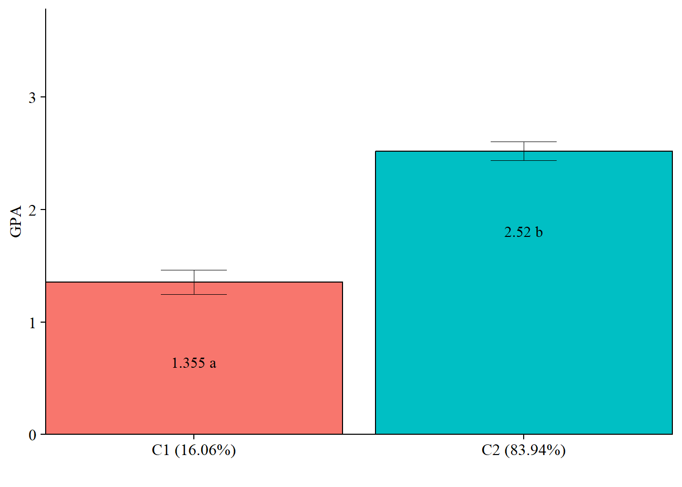
check=TRUE, run = TRUE, hashfilename = FALSE)17.2.1.2 Plot Distal Outcome mean differences
modelParams <- readModels(here("three_step", "auto_3step", "c2_du3step.out"))

# Extract class size
c_size <- as.data.frame(modelParams[["class_counts"]][["modelEstimated"]][["proportion"]]) %>%
  rename("cs" = 1) %>%
  mutate(cs = round(cs*100, 2))

c_size_val <- paste0("C", 1:nrow(c_size), glue(" ({c_size[1:nrow(c_size),]}%)"))


# Extract information as data frame
estimates <- as.data.frame(modelParams[["lcCondMeans"]][["overall"]]) %>%
  reshape2::melt(id.vars = "var") %>%
  mutate(variable = as.character(variable),
         LatentClass = case_when(
           endsWith(variable, "1") ~ c_size_val[1],
           endsWith(variable, "2") ~ c_size_val[2])) %>% #Add to this based on the number of classes you have
  head(-3) %>%
  pivot_wider(names_from = variable, values_from = value) %>%
  unite("mean", contains("m"), na.rm = TRUE) %>%
  unite("se", contains("se"), na.rm = TRUE) %>%
  mutate(across(c(mean, se), as.numeric))

# Add labels (NOTE: You must change the labels to match the significance testing!!)
value_labels <- paste0(estimates$mean, c(" a"," b"))

# Plot bar graphs
estimates %>%
  ggplot(aes(fill = LatentClass, y = mean, x = LatentClass)) +
  geom_bar(position = "dodge", stat = "identity", color = "black") +
  geom_errorbar(aes(ymin=mean-se, ymax=mean+se),
                size=.3,
                width=.2,
                position=position_dodge(.9)) +
  geom_text(aes(y = mean, label = value_labels),
            family = "serif", size = 4,
            position=position_dodge(.9),
            vjust = 8) +
  #scale_fill_grey(start = .5, end = .7) +
  labs(y="GPA", x="") +
  theme_cowplot() +
  theme(text = element_text(family = "serif", size = 12),
        axis.text.x = element_text(size=12),
        legend.position="none") +
  coord_cartesian(expand = FALSE,
                  ylim=c(0,max(estimates$mean*1.5))) # Change ylim based on distal outcome rang