13 Manual 3-Step Covariate Only

Data source:

The first examples utilizes the public-use dataset, The Longitudinal Survey of American Youth (LSAY): See documentation here
The second example utilizes a dataset on undergraduate Cheating available from the poLCA package (Dayton, 1998): See documentation here

13.1 Load packages

library(MplusAutomation)
library(tidyverse) #collection of R packages designed for data science
library(here) #helps with filepaths
library(janitor) #clean_names
library(gt) # create tables
library(cowplot) # a ggplot theme
library(DiagrammeR) # create path diagrams
library(glue) # allows us to paste expressions into R code
library(data.table) # used for `melt()` function  
library(poLCA)
library(reshape2)

Our example is Mother’s Education as a predictor of latent class membership of Math Attitudes

Application: Longitudinal Study of American Youth, Science Attitudes

Name	Variable Description
LCA Indicators & Auxiliary Variables: Math Attitudes Example


enjoy	I enjoy math.
useful	Math is useful in everyday problems.
logical	Math helps a person think logically.
job	It is important to know math to get a good job.
adult	I will use math in many ways as an adult.
Auxiliary Variables
mothed	Level of education: (1) less than high school, (2) high school diploma, (3) some college, (4) 4-year college, and (5) an advanced degree.

The data can be found in the data folder and is called lsay_subset.csv.

lsay_data <- read_csv(here("three_step","data","lsay_subset.csv")) %>% 
  clean_names() %>%   # make variable names lowercase
  mutate(female = recode(gender, `1` = 0, `2` = 1)) # relabel values from 1,2 to 0,1

13.2 Descriptive Statistics

dframe <- lsay_data %>%
  pivot_longer(
    c(enjoy, useful, logical, job, adult),
    names_to = "Variable"
  ) %>%
  group_by(Variable) %>%
  summarise(
    Count = sum(value == 1, na.rm = TRUE),
    Total = n(),
    .groups = "drop"
  ) %>%
  mutate(`Proportion Endorsed` = round(Count / Total, 3)) %>%
  dplyr::select(Variable, `Proportion Endorsed`, Count)

gt(dframe) %>%
  tab_header(
    title = md("**LCA Indicator Endorsement**"),
    subtitle = md("&nbsp;")
  ) %>%
  tab_options(
    column_labels.font.weight = "bold",
    row_group.font.weight = "bold"
  )

Variable	Proportion Endorsed	Count
LCA Indicator Endorsement

adult	0.596	1858
enjoy	0.573	1784
job	0.625	1947
logical	0.541	1686
useful	0.589	1835

Mother’s Education

summary(factor(lsay_data$mothed))
#>    1    2    3    4    5 NA's 
#>  452 1732  304  368  158  102

13.3 Manual ML Three-step

13.3.1 Step 1 - Class Enumeration w/ Auxiliary Specification

This step is done after class enumeration (or after you have selected the best latent class model). In this example, the four class model was the best. Now, we re-estimate the four-class model using optseed for efficiency. The difference here is the SAVEDATA command, where I can save the posterior probabilities and the modal class assignment that will be used in steps two and three.


step1  <- mplusObject(
  TITLE = "Step 1 - Three-Step using LSAL", 
  VARIABLE = 
  "categorical = enjoy useful logical job adult; 
   usevar = enjoy useful logical job adult;
    
   classes = c(4); 
    
   auxiliary =  mothed  ! covariate ",
  
  ANALYSIS = 
   "estimator = mlr; 
    type = mixture;
    starts = 0;
    optseed = 568405;",
  
  SAVEDATA = 
   "File=savedata_cov.dat;
    Save=cprob;",
  
  OUTPUT = "residual tech11 tech14",
  
  PLOT = 
    "type = plot3; 
    series = enjoy-adult(*);",
  
  usevariables = colnames(lsay_data),
  rdata = lsay_data)

step1_fit <- mplusModeler(step1,
                            dataout=here("three_step", "manual_3step", "Step1.dat"),
                            modelout=here("three_step", "manual_3step", "one_cov.inp") ,
                            check=TRUE, run = TRUE, hashfilename = FALSE)

source(here("functions", "plot_lca.R"))
output_lsay <- readModels(here("three_step", "manual_3step","one_cov.out"))

plot_lca(model_name = output_lsay)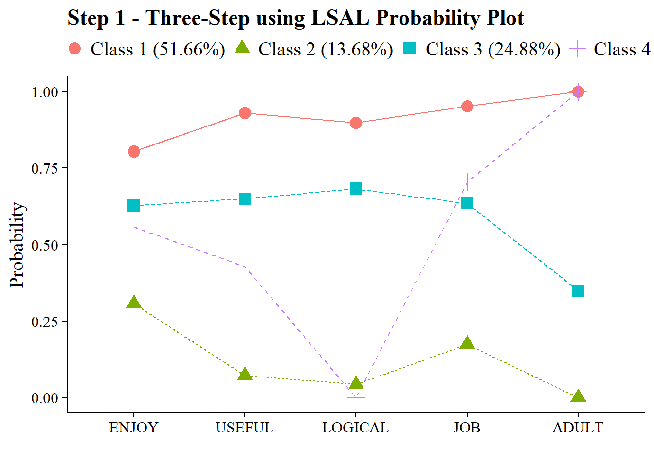

13.3.2 Step 2 - Determine Measurement Error

Extract logits for the classification probabilities for the most likely latent class

logit_cprobs <- as.data.frame(output_lsay[["class_counts"]]
                                       [["logitProbs.mostLikely"]])

Extract saved dataset which is part of the mplusObject “step1_fit”

savedata <- as.data.frame(output_lsay[["savedata"]])

Rename the column in savedata named “C” and change to “N”

colnames(savedata)[colnames(savedata)=="C"] <- "N"

13.3.3 Step 3 - LCA Auxiliary Variable Model with 1 Covariate

step3  <- mplusObject(
  TITLE = "Step3 - 3step LSAY", 
  
  VARIABLE = 
 "nominal=N;
  usevar = n;
  
  classes = c(4);
  
  usevar = mothed;" ,
  
  ANALYSIS = 
 "estimator = mlr; 
  type = mixture; 
  starts = 0;",
 
  DEFINE = 
   "center mothed (grandmean);",
  
  MODEL =
  glue(
 " %OVERALL%
 
  C on mothed;        ! covariate as predictor of C

     %C#1%
  [n#1@{logit_cprobs[1,1]}]; ! MUST EDIT if you do not have a 4-class model. 
  [n#2@{logit_cprobs[1,2]}];
  [n#3@{logit_cprobs[1,3]}];

  %C#2%
  [n#1@{logit_cprobs[2,1]}];
  [n#2@{logit_cprobs[2,2]}];
  [n#3@{logit_cprobs[2,3]}];

  
  %C#3%
  [n#1@{logit_cprobs[3,1]}];
  [n#2@{logit_cprobs[3,2]}];
  [n#3@{logit_cprobs[3,3]}];


  %C#4%
  [n#1@{logit_cprobs[4,1]}];
  [n#2@{logit_cprobs[4,2]}];
  [n#3@{logit_cprobs[4,3]}];"),
  
 
  usevariables = colnames(savedata), 
  rdata = savedata)

step3_fit <- mplusModeler(step3,
               dataout=here("three_step", "manual_3step", "Step3.dat"), 
               modelout=here("three_step", "manual_3step", "three_cov.inp"), 
               check=TRUE, run = TRUE, hashfilename = FALSE)

13.3.3.1 Covariates Relations

modelParams <- readModels(here("three_step", "manual_3step", "three_cov.out"))

# Extract information as data frame
cov <- as.data.frame(modelParams[["parameters"]][["unstandardized"]]) %>%
   filter(str_detect(paramHeader, "^C#\\d+\\.ON$")) %>% 
#  mutate(param = str_replace(param, "FEMALE", "Gender")) %>% # Change this to your own covariates
  mutate(param = str_replace(param, "MOTHED", "Mother's Education")) %>%
  mutate(est = format(round(est, 3), nsmall = 3),
         se = round(se, 2),
         pval = round(pval, 3)) %>% 
  mutate(latent_class = str_replace(paramHeader, "^C#(\\d+)\\.ON$", "Class \\1")) %>% 
  dplyr::select(param, est, se, pval, latent_class) %>% 
  mutate(se = paste0("(", format(round(se,2), nsmall =2), ")")) %>% 
  unite(logit, est, se, sep = " ") %>% 
  dplyr::select(param, logit, pval, latent_class) %>% 
  mutate(pval = ifelse(pval<0.001, paste0("<.001*"),
                       ifelse(pval<0.05, paste0(scales::number(pval, accuracy = .001), "*"),
                              scales::number(pval, accuracy = .001)))) 

or <- as.data.frame(modelParams[["parameters"]][["odds"]]) %>%
  filter(str_detect(paramHeader, "^C#\\d+\\.ON$")) %>% 
 # mutate(param = str_replace(param, "FEMALE", "Gender")) %>% # Change this to your own covariates
  mutate(param = str_replace(param, "MOTHED", "Mother's Education")) %>%
  mutate(est = format(round(est, 3), nsmall = 3)) %>% 
  mutate(latent_class = str_replace(paramHeader, "^C#(\\d+)\\.ON$", "Class \\1")) %>% 
  mutate(CI = paste0("[", format(round(lower_2.5ci, 3), nsmall = 3), ", ", format(round(upper_2.5ci, 3), nsmall = 3), "]")) %>% 
  dplyr::select(param, est, CI, latent_class) %>% 
  rename(or = est)
  
combined <- or %>% 
  full_join(cov) %>% 
  dplyr::select(param, latent_class, logit, pval, or, CI)


# Create table

combined %>% 
  gt(groupname_col = "latent_class", rowname_col = "param") %>%
  tab_header(
    title = "Covariate Results: Mother's Education on Class") %>%
  cols_label(
    logit = md("Logit (*se*)"),
    or = md("Odds Ratio"),
    CI = md("95% CI"),
    pval = md("*p*-value")) %>% 
  sub_missing(1:3,
              missing_text = "") %>%
  sub_values(values = c("999.000"), replacement = "-") %>% 
  cols_align(align = "center") %>% 
  opt_align_table_header(align = "left") %>% 
  gt::tab_options(table.font.names = "serif") %>%   
  tab_footnote(
    footnote = "Reference Class: 4",
    locations = cells_title(groups = "title")
  )

	Logit (se)	p-value	Odds Ratio	95% CI
Covariate Results: Mother's Education on Class¹
Class 1
Mother's Education	0.269 (0.10)	0.007*	1.309	[1.078, 1.589]
Class 2
Mother's Education	0.158 (0.11)	0.156	1.171	[0.942, 1.457]
Class 3
Mother's Education	0.237 (0.11)	0.035*	1.268	[1.017, 1.580]
¹ Reference Class: 4

13.4 Automated Three-Step

Application: Undergraduate Cheating behavior

“Dichotomous self-report responses by 319 undergraduates to four questions about cheating behavior” (poLCA, 2016).

Prepare data


data(cheating)

cheating <- cheating %>% clean_names() 

df_cheat <-  cheating %>%                                  
  dplyr::select(1:4) %>%                                  
  mutate_all(funs(.-1)) %>%                                
  mutate(gpa = cheating$gpa)

# Detaching packages that mask the dpylr functions 
detach(package:poLCA, unload = TRUE)
detach(package:MASS, unload = TRUE)

13.4.1 R3STEP

R3STEP incorporates latent class predictors with mixture models. However, it is recommended to use the manual three-step.

13.4.1.1 Run the R3STEP model with `gpa` as the latent class predictor


m_stepr  <- mplusObject(
  TITLE = "R3STEP - GPA as Predictor", 
  VARIABLE = 
   "categorical = lieexam-copyexam; 
    usevar = lieexam-copyexam;
    auxiliary = gpa (R3STEP);
    classes = c(2);",
  
  ANALYSIS = 
   "estimator = mlr; 
    type = mixture;
    starts = 500 100; 
    processors = 10;",
  
  OUTPUT = "sampstat patterns tech11 tech14;",
  
  PLOT = 
    "type = plot3; 
     series = lieexam-copyexam(*);",
  
  usevariables = colnames(df_cheat),
  rdata = df_cheat)

m_stepr_fit <- mplusModeler(m_stepr, 
                            dataout=here("three_step", "auto_3step", "r3step.dat"),
                            modelout=here("three_step", "auto_3step", "c2_r3step.inp") ,
                            check=TRUE, run = TRUE, hashfilename = FALSE)

13.4.1.2 Regression slopes and odds ratios

TESTS OF CATEGORICAL LATENT VARIABLE MULTINOMIAL LOGISTIC REGRESSIONS USING
THE 3-STEP PROCEDURE

   WARNING:  LISTWISE DELETION IS APPLIED TO THE AUXILIARY VARIABLES IN THE
   ANALYSIS.  TO AVOID LISTWISE DELETION, DATA IMPUTATION CAN BE USED
   FOR THE AUXILIARY VARIABLES FOLLOWED BY ANALYSIS WITH TYPE=IMPUTATION.
   NUMBER OF DELETED OBSERVATIONS:  4
   NUMBER OF OBSERVATIONS USED:  315

                                                    Two-Tailed
                    Estimate       S.E.  Est./S.E.    P-Value

 C#1        ON
    GPA               -0.698      0.255     -2.739      0.006

 Intercepts
    C#1               -0.241      0.460     -0.523      0.601

Parameterization using Reference Class 1

 C#2        ON
    GPA                0.698      0.255      2.739      0.006

 Intercepts
    C#2                0.241      0.460      0.523      0.601


ODDS RATIOS FOR TESTS OF CATEGORICAL LATENT VARIABLE MULTINOMIAL LOGISTIC REGRESSIONS
USING THE 3-STEP PROCEDURE

                                                95% C.I.
                    Estimate       S.E. Lower 2.5% Upper 2.5%

 C#1        ON
    GPA                0.498      0.127      0.302      0.820


Parameterization using Reference Class 1

 C#2        ON
    GPA                2.009      0.512      1.220      3.310

12 Class Separation

14 Manual 3-Step Distal Only