6 Polytomous LCA

Polytomous LCA deals with variables that have more than two categories, such as survey questions with responses like never, sometimes, and always. The workflow of a polytomous LCA model is similar to that of an LCA model with binary indicators. However, polytomous LCA captures more complex response patterns, which can make interpretation a bit trickier. The following code demonstrates an example, along with a visualization of the model.

---

6.1 Example: Elections

“Two sets of six questions with four responses each, asking respondents’ opinions of how well various traits describe presidential candidates Al Gore and George W. Bush. Also potential covariates vote choice, age, education, gender, and party ID. Source: The National Election Studies (2000).” (poLCA, 2016) See documentation here

Two sets of six questions with four responses each, asking respondents’ opinions of how well various traits describe presidential candidates Al Gore and George W. Bush. In the election data set, respondents to the 2000 American National Election Study public opinion poll were asked to evaluate how well a series of traits—moral, caring, knowledgeable, good leader, dishonest, and intelligent—described presidential candidates Al Gore and George W. Bush. Each question had four possible choices: (1) extremely well; (2) quite well; (3) not too well; and (4) not well at all.

---

Load packages

library(poLCA)
library(tidyverse)
library(janitor)
library(gt)
library(MplusAutomation)
library(here)
library(glue)

---

6.2 Prepare Data

data(election)

# Detaching packages that mask the dpylr functions 
detach(package:poLCA, unload = TRUE)
detach(package:MASS, unload = TRUE)

df_election <-  election %>% 
  clean_names() %>% 
  select(moralb:intelb) %>% 
  mutate(across(everything(), 
                ~ as.factor(as.numeric(gsub("\\D", "", .))), 
                .names = "{.col}1")) 

# Quick summary
summary(df_election)
#>                moralb                  caresb   
#>  1 Extremely well :340   1 Extremely well :155  
#>  2 Quite well     :841   2 Quite well     :625  
#>  3 Not too well   :330   3 Not too well   :562  
#>  4 Not well at all: 98   4 Not well at all:342  
#>  NA's             :176   NA's             :101  
#>                knowb                   leadb    
#>  1 Extremely well :274   1 Extremely well :266  
#>  2 Quite well     :933   2 Quite well     :842  
#>  3 Not too well   :379   3 Not too well   :407  
#>  4 Not well at all:133   4 Not well at all:166  
#>  NA's             : 66   NA's             :104  
#>               dishonb                  intelb    moralb1   
#>  1 Extremely well : 70   1 Extremely well :329   1   :340  
#>  2 Quite well     :288   2 Quite well     :967   2   :841  
#>  3 Not too well   :653   3 Not too well   :306   3   :330  
#>  4 Not well at all:574   4 Not well at all:110   4   : 98  
#>  NA's             :200   NA's             : 73   NA's:176  
#>  caresb1     knowb1     leadb1    dishonb1   intelb1   
#>  1   :155   1   :274   1   :266   1   : 70   1   :329  
#>  2   :625   2   :933   2   :842   2   :288   2   :967  
#>  3   :562   3   :379   3   :407   3   :653   3   :306  
#>  4   :342   4   :133   4   :166   4   :574   4   :110  
#>  NA's:101   NA's: 66   NA's:104   NA's:200   NA's: 73

---

6.3 Descriptive Statistics

ds <- df_election %>% 
  pivot_longer(moralb1:intelb1, names_to = "variable") %>% 
  count(variable, value) %>%  # Count occurrences of each value for each variable
  group_by(variable) %>%
  mutate(prop = n / sum(n)) %>% 
  arrange(desc(variable))

# Create the table
prop_table <- ds %>% 
  gt() %>% 
  tab_header(title = md("**Descriptive Summary**")) %>%
  cols_label(
    variable = "Variable",
    n = md("*N*"),
    prop = md("Proportion")
  ) %>%
  fmt_number(c("n", "prop"), decimals = 2) %>%  # Format both n and prop columns
  cols_align(
    align = "center",
    columns = c(prop, n)
  ) 

# View the table
prop_table

Descriptive Summary
value	N	Proportion
moralb1
1	340.00	0.19
2	841.00	0.47
3	330.00	0.18
4	98.00	0.05
NA	176.00	0.10
leadb1
1	266.00	0.15
2	842.00	0.47
3	407.00	0.23
4	166.00	0.09
NA	104.00	0.06
knowb1
1	274.00	0.15
2	933.00	0.52
3	379.00	0.21
4	133.00	0.07
NA	66.00	0.04
intelb1
1	329.00	0.18
2	967.00	0.54
3	306.00	0.17
4	110.00	0.06
NA	73.00	0.04
dishonb1
1	70.00	0.04
2	288.00	0.16
3	653.00	0.37
4	574.00	0.32
NA	200.00	0.11
caresb1
1	155.00	0.09
2	625.00	0.35
3	562.00	0.31
4	342.00	0.19
NA	101.00	0.06

# Save as a Word doc
#gtsave(prop_table, here("figures", "prop_table.docx"))

---

6.4 Enumeration

This code uses the mplusObject function in the MplusAutomation package.

lca_enumeration  <- lapply(1:6, function(k) {
  lca_enum  <- mplusObject(
      
    TITLE = glue("{k}-Class"), 
  
    VARIABLE = glue(
    "categorical = moralb1-intelb1; 
     usevar = moralb1-intelb1;
     classes = c({k}); "),
  
  ANALYSIS = 
   "estimator = mlr; 
    type = mixture;
    starts = 500 100; 
    processors = 10;",
  
  OUTPUT = "sampstat residual tech11 tech14 svalues;",

  
  usevariables = colnames(df_election),
  rdata = df_election)

lca_enum_fit <- mplusModeler(lca_enum, 
                            dataout=glue(here("poLCA", "election.dat")),
                            modelout=glue(here("poLCA", "c{k}_election.inp")) ,
                            check=TRUE, run = TRUE, hashfilename = FALSE)
})

---

6.4.1 Table of Fit

source(here("functions","enum_table.R"))

output_election <- readModels(here("poLCA"), filefilter = "election", quiet = TRUE)

# To see rows:
#seeRows(output_election)

# Arguments for `enum_table`
# 1. readModels objects
# 2-5. Rows of successfully estimated models 
fit_table <- enum_table(output_election, 1:6)
fit_table

Model Fit Summary Table1
Classes	Par	LL	BIC	aBIC	CAIC	AWE	BLRT	VLMR	BF	cmPk
1-Class	18	−11,838.63	23,811.84	23,754.66	23,829.84	24,000.42	–	–	0.0	<.001
2-Class	37	−10,680.33	21,637.30	21,519.75	21,674.30	22,024.92	<.001	<.001	0.0	<.001
3-Class	56	−10,184.89	20,788.46	20,610.55	20,844.46	21,375.14	<.001	<.001	0.0	<.001
4-Class	75	−9,979.58	20,519.89	20,281.62	20,594.89	21,305.63	<.001	<.001	0.0	<.001
5-Class	94	−9,863.42	20,429.62	20,130.99	20,523.62	21,414.41	<.001	<.001	>100	1.000
6-Class	113	−9,809.63	20,464.09	20,105.10	20,577.09	21,647.93	<.001	0.629	–	<.001
1 Note. Par = Parameters; LL = model log likelihood; BIC = Bayesian information criterion; aBIC = sample size adjusted BIC; CAIC = consistent Akaike information criterion; AWE = approximate weight of evidence criterion; BLRT = bootstrapped likelihood ratio test p-value; cmPk = approximate correct model probability.

---

Save table:

gtsave(fit_table, here("figures", "fit_table.png"))

---

6.4.2 Information Criteria Plot

ic_plot(output_election)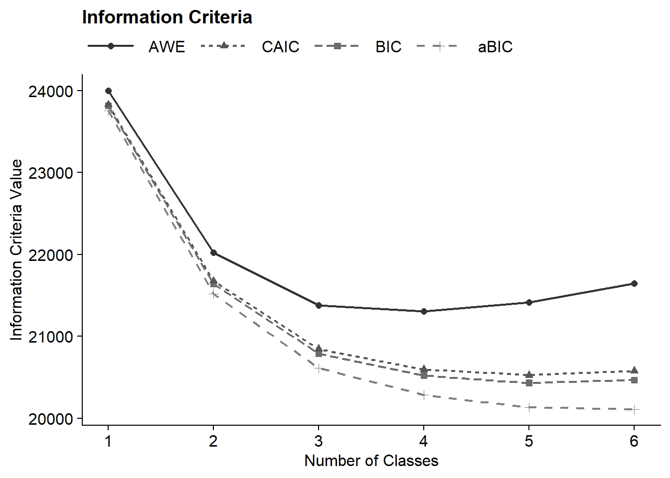

---

Save figure:

ggsave(here("figures", "info_criteria.png"), dpi="retina", bg = "white", height=5, width=7, units="in")

---

6.4.3 4-Class Probability Plot

The functions poLCA_stacked and poLCA_grouped create visualizations of class probabilities for LCA with polytomous indicators. Each function takes the following arguments:

• model_name: The LCA model read into R using the readModels function from the MplusAutomation package.
• category_labels: A character vector of category labels for the response options (e.g., survey answers).

Note: Double check that the labels are in the correct order!

source(here("functions","poLCA_plot.R"))

poLCA_stacked(output_election$c5_election.out, category_labels = c("1" = "1: Extremely well", 
                                                                   "2" = "2: Quite Well", 
                                                                   "3" = "3: Not Too Well", 
                                                                   "4" = "4: Not Well at All"))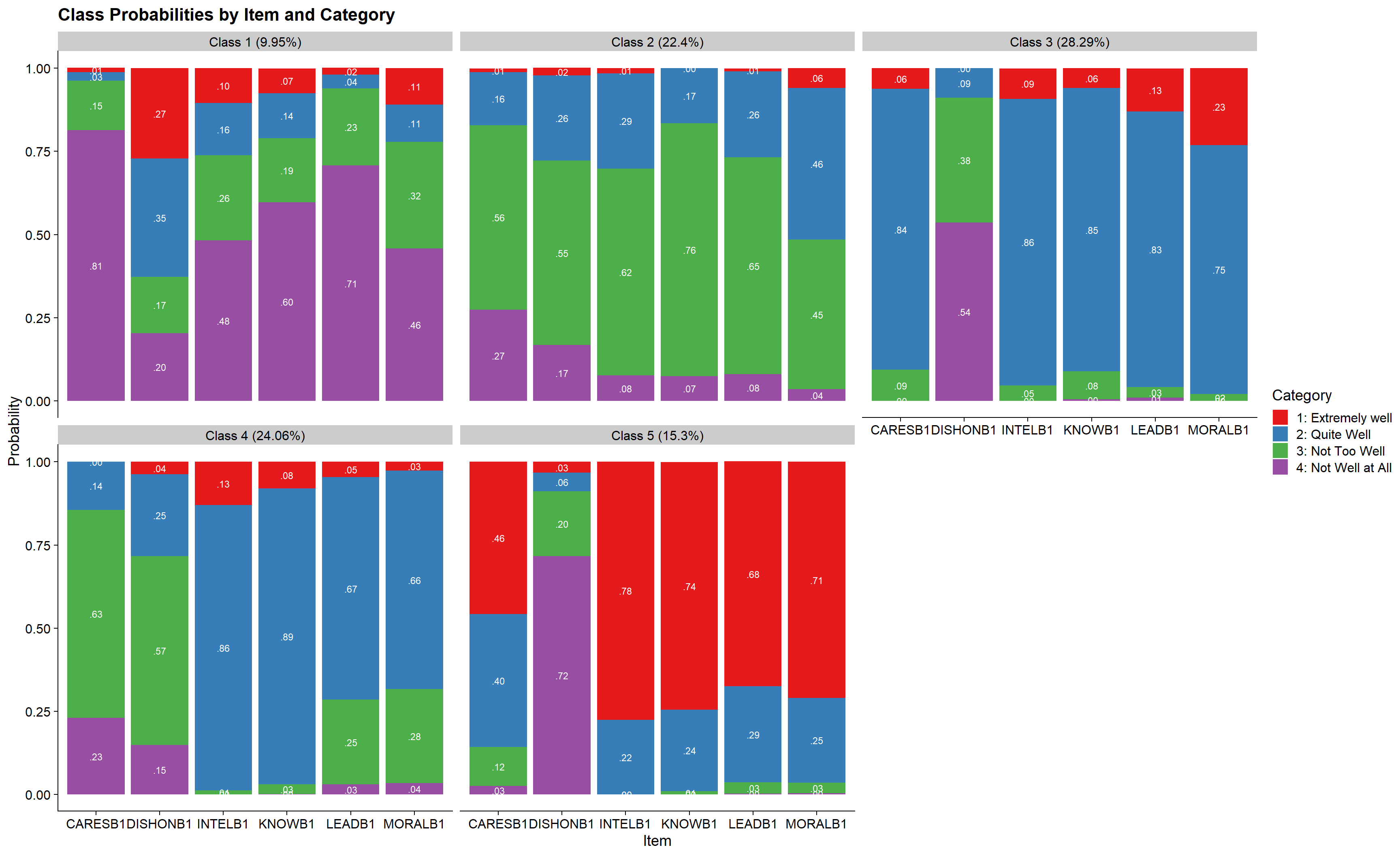

Alternative plot

poLCA_grouped(output_election$c5_election.out, category_labels = c("1" = "1: Extremely well", 
                                                                   "2" = "2: Quite Well", 
                                                                   "3" = "3: Not Too Well", 
                                                                   "4" = "4: Not Well at All"))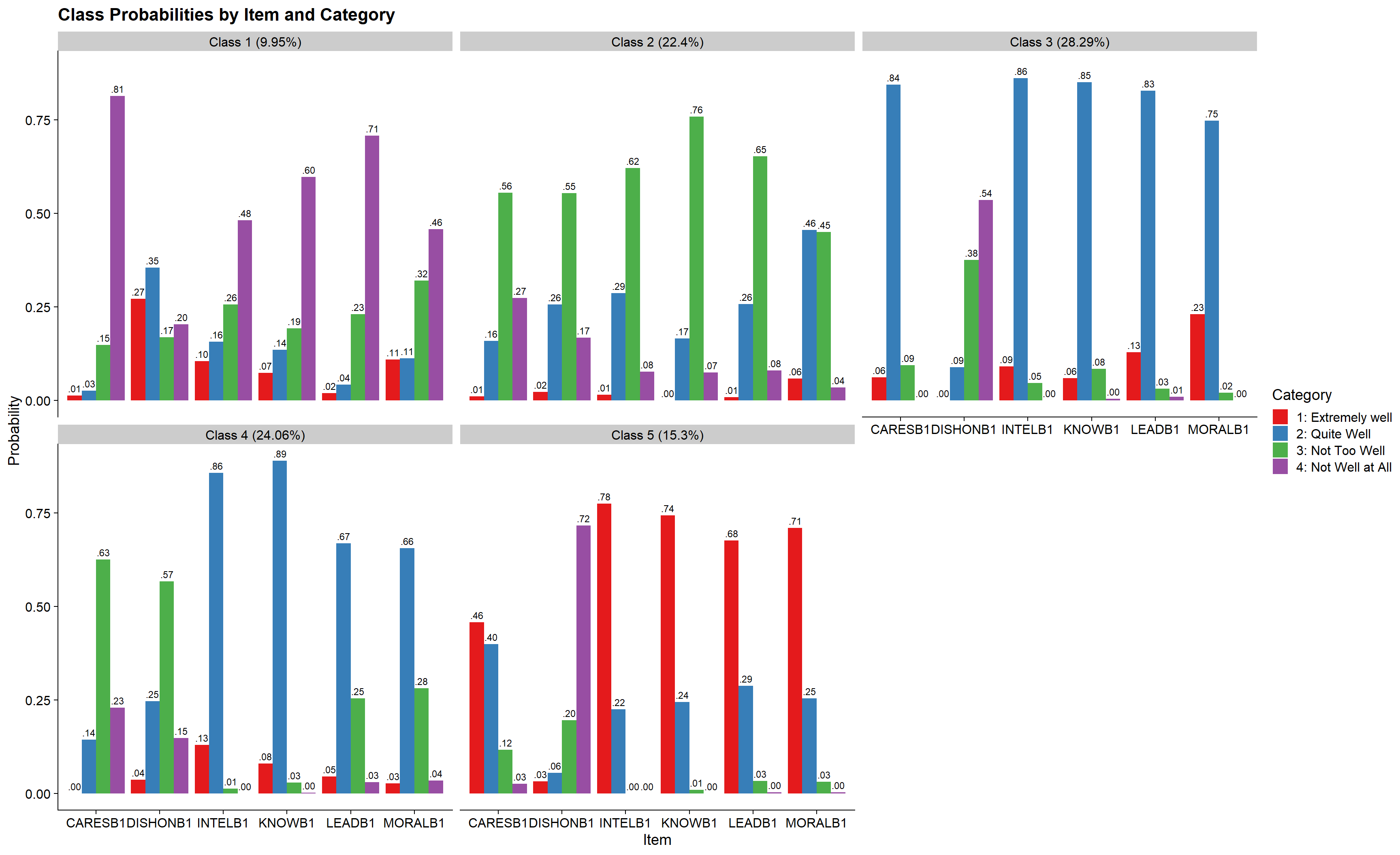

---

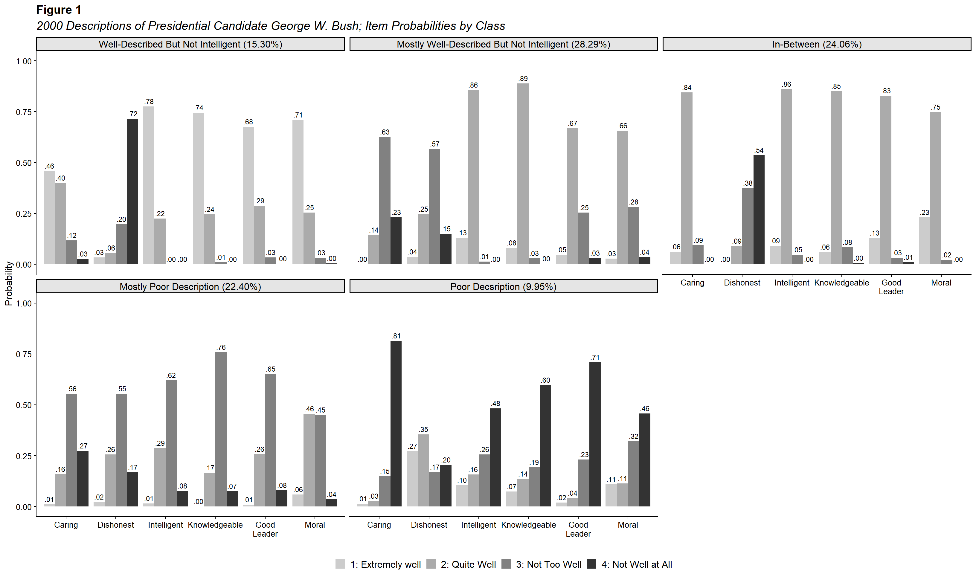
6.4.4 APA-formatted Plot

# Model 
model <- output_election$c5_election.out


# Title
title <- "2000 Descriptions of Presidential Candidate George W. Bush; Item Probabilities by Class"

# Item names
item_labels <- c("CARESB1" = "Caring",
                 "DISHONB1" = "Dishonest",
                 "INTELB1" = "Intelligent",
                 "KNOWB1" = "Knowledgeable",
                 "LEADB1" = "Good Leader",
                 "MORALB1" = "Moral")

# Item Category
category_labels <- c("1" = "1: Extremely well", 
                     "2" = "2: Quite Well", 
                     "3" = "3: Not Too Well", 
                     "4" = "4: Not Well at All")

# Class labels
class_labels <- c("1" = "Poor Decsription (9.95%)",
                  "2" = "Mostly Poor Description (22.40%)",
                  "3" = "In-Between (24.06%)",
                  "4" = "Mostly Well-Described But Not Intelligent (28.29%)",
                  "5" = "Well-Described But Not Intelligent (15.30%)")


#### END EDIT ####

6.4.4.1 Extract data needed for plotting

# Extract data needed for plotting 
plot_data <- data.frame(model$parameters$probability.scale) %>%
  dplyr::select(est, LatentClass, param, category) %>%
  mutate(
    items = factor(param, labels = item_labels),
    class = factor(LatentClass, labels = class_labels),
    cat = factor(category, labels = category_labels)
  ) %>% 
  mutate(class = factor(class, levels = rev(levels(factor(class))))) 

---

6.4.4.2 Final grouped bar plot

## Plot data
plot_data %>%
  ggplot(aes(
    x = items,
    y = est,
    fill = cat,
    group = cat
  )) +
  geom_bar(stat = "identity", position = "dodge") +
  geom_text(aes(label = sub("^0\\.", ".", sprintf("%.2f", est))), 
            position = position_dodge(width = 0.9), 
            vjust = -0.5, size = 3) +
  facet_wrap(~ class) + 
  ylim(0, 1) +
  scale_x_discrete(
    "",
    labels = function(x)
      str_wrap(x, width = 10)
  ) +
  labs(title = "Figure 1",
       subtitle = title,
       y = "Probability") +
  theme_bw(12) +
  scale_fill_grey(start = 0.8, end = 0.2) + # Gives different shades
  theme(
    text = element_text(family = "sans", size = 12),
    legend.text = element_text(family = "sans", size = 12, color = "black"),
    legend.title = element_blank(),
    legend.position = "bottom",
    legend.justification = "center", 
    axis.text.x = element_text(vjust = 1),
    plot.subtitle = element_text(face = "italic", size = 15),
    plot.title = element_text(size = 15),
    strip.background = element_rect(fill = "grey90", color = "black", size = 1),
    strip.text = element_text(size = 12)
  ) 

---

Save figure:

ggsave(here("figures", "APA_plot1.png"), dpi="retina", bg = "white", height=9, width=15, units="in")

---

6.4.4.3 Alternative

## Plot data
plot_data %>%
  ggplot(aes(
    x = items,
    y = est,
    fill = cat,
    group = cat
  )) +
  geom_bar(stat = "identity", position = "dodge") +
  geom_text(aes(label = sub("^0\\.", ".", sprintf("%.2f", est))), 
            position = position_dodge(width = 0.9), 
            vjust = -0.5, size = 3) +
  facet_wrap(~ class) + 
  ylim(0, 1) +
  scale_x_discrete(
    "",
    labels = function(x)
      str_wrap(x, width = 10)
  ) +
  labs(title = "Figure 1",
       subtitle = title,
       y = "Probability") +
  theme_cowplot(12) +
  scale_fill_grey(start = 0.8, end = 0.2) + # Gives different shades
  theme(
    text = element_text(family = "sans", size = 12),
    legend.text = element_text(family = "sans", size = 12, color = "black"),
    legend.title = element_blank(),
    legend.position = "bottom",
    legend.justification = "center", 
    axis.text.x = element_text(vjust = 1),
    plot.subtitle = element_text(face = "italic", size = 15),
    plot.title = element_text(size = 15),
    strip.background = element_rect(fill = "grey90", color = "black", size = 1),
    strip.text = element_text(size = 12)
  )

---

Save figure:

ggsave(here("figures", "APA_plot2.png"), dpi="retina", bg = "white", height=10, width=17, units="in")