8 Latent Transition Analysis
Data Source: The data used to illustrate these analyses include elementary school student Science Attitude survey items collected during 7th and 10th grades from the Longitudinal Study of American Youth (LSAY; Miller, 2015).
To install package {rhdf5}
if (!requireNamespace("BiocManager", quietly = TRUE))
  install.packages("BiocManager")

#BiocManager::install("rhdf5")
Load packages
library(MplusAutomation)
library(rhdf5)
library(tidyverse)
library(here)
library(glue)
library(janitor)
library(gt)
library(reshape2)
library(cowplot)
library(ggrepel)
library(haven)
library(modelsummary)
library(corrplot)
library(DiagrammeR)
library(filesstrings)
library(PNWColors)
Read in LSAY data file, lsay_new.csv.
lsay_data <- read_csv(here("data","lsay_lta.csv"), na = c("9999")) %>%
    mutate(across(everything(), as.numeric))
8.1 Descriptive Statistics
8.1.1 Data Summary
data <- lsay_data

select_data <- data %>%
 select(female, minority, ab39m:ga33l)

f <- All(select_data) ~ Mean + SD + Min + Median + Max + Histogram
datasummary(f, data, output="markdown")| Mean | SD | Min | Median | Max | Histogram | |
|---|---|---|---|---|---|---|
| female | 0.48 | 0.50 | 0.00 | 0.00 | 1.00 | ▇▆ |
| minority | 0.23 | 0.42 | 0.00 | 0.00 | 1.00 | ▇▂ |
| ab39m | 0.61 | 0.49 | 0.00 | 1.00 | 1.00 | ▄▇ |
| ab39t | 0.40 | 0.49 | 0.00 | 0.00 | 1.00 | ▇▅ |
| ab39u | 0.49 | 0.50 | 0.00 | 0.00 | 1.00 | ▇▇ |
| ab39w | 0.40 | 0.49 | 0.00 | 0.00 | 1.00 | ▇▅ |
| ab39x | 0.46 | 0.50 | 0.00 | 0.00 | 1.00 | ▇▆ |
| ga33a | 0.58 | 0.49 | 0.00 | 1.00 | 1.00 | ▅▇ |
| ga33h | 0.43 | 0.49 | 0.00 | 0.00 | 1.00 | ▇▅ |
| ga33i | 0.51 | 0.50 | 0.00 | 1.00 | 1.00 | ▇▇ |
| ga33k | 0.42 | 0.49 | 0.00 | 0.00 | 1.00 | ▇▅ |
| ga33l | 0.42 | 0.49 | 0.00 | 0.00 | 1.00 | ▇▅ |
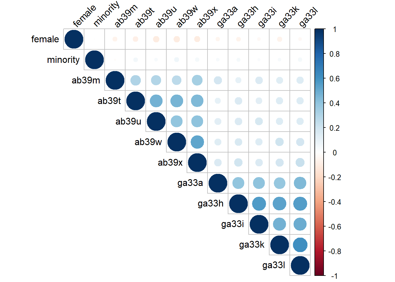
8.1.2 Correlation Table
select_data %>%
datasummary_correlation(output = "markdown")| female | minority | ab39m | ab39t | ab39u | ab39w | ab39x | ga33a | ga33h | ga33i | ga33k | ga33l | |
|---|---|---|---|---|---|---|---|---|---|---|---|---|
| female | 1 | . | . | . | . | . | . | . | . | . | . | . |
| minority | -.01 | 1 | . | . | . | . | . | . | . | . | . | . |
| ab39m | -.06 | -.01 | 1 | . | . | . | . | . | . | . | . | . |
| ab39t | -.09 | .05 | .30 | 1 | . | . | . | . | . | . | . | . |
| ab39u | -.11 | .03 | .30 | .48 | 1 | . | . | . | . | . | . | . |
| ab39w | -.11 | .06 | .27 | .46 | .40 | 1 | . | . | . | . | . | . |
| ab39x | -.11 | .05 | .33 | .45 | .41 | .52 | 1 | . | . | . | . | . |
| ga33a | -.05 | .04 | .19 | .11 | .13 | .13 | .15 | 1 | . | . | . | . |
| ga33h | -.06 | .04 | .10 | .15 | .16 | .16 | .20 | .40 | 1 | . | . | . |
| ga33i | -.04 | .02 | .15 | .13 | .18 | .15 | .16 | .40 | .57 | 1 | . | . |
| ga33k | -.07 | .04 | .13 | .15 | .15 | .20 | .18 | .39 | .54 | .48 | 1 | . |
| ga33l | -.04 | .05 | .15 | .15 | .14 | .18 | .23 | .44 | .56 | .49 | .62 | 1 |
8.2 Enumeration
8.2.1 Enumerate Time Point 1 (7th grade)
# NOTE CHANGE: '1:6' indicates the number of k-class models to estimate
# User can change this number to fit research context
# In this example, the code loops or iterates over values 1 through 6 ( '{k}' )
#
t1_enum_k_16  <- lapply(1:6, function(k) {
  enum_t1  <- mplusObject(

# The 'glue' function inserts R code within a string or "quoted green text" using the syntax {---}
#
    TITLE = glue("Class-{k}_Time1"),

    VARIABLE = glue(
    "!!! NOTE CHANGE: List of the five 7th grade science attitude indicators !!!
     categorical = ab39m-ab39x;
          usevar = ab39m-ab39x;

     classes = c({k});"),

  ANALYSIS =
   "estimator = mlr;
    type = mixture;
    !!! NOTE CHANGE: The intial and final start values. Reduce to speed up estimation time. !!!
    starts = 500 100;
    processors=10;",

  OUTPUT = "sampstat residual tech11 tech14;",

  PLOT =
    "type = plot3;
    series = ab39m-ab39x(*);",

  usevariables = colnames(lsay_data),
  rdata = lsay_data)

# NOTE CHANGE: Fix to match appropriate sub-folder name
# See after `here` function (e.g., "enum_LCA_time1")
enum_t1_fit <- mplusModeler(enum_t1,
                 dataout=here("lta","enum_t1","t1.dat"),
                 modelout=glue(here("lta","enum_t1","c{k}_lca_enum_time1.inp")),
                 check=TRUE, run = TRUE, hashfilename = FALSE)
})
NEXT STEP Check the output (.out) files to check for convergence warnings or syntax errors.
8.2.2 Enumerate Time Point 2 (10th grade)
t2_enum_k_16  <- lapply(1:6, function(k) {
  enum_t2  <- mplusObject(

    TITLE = glue("Class-{k}_Time2"),

    VARIABLE =
  glue(
    "!!! NOTE CHANGE: List of the five 10th grade science attitude indicators !!!
     categorical = ga33a-ga33l;
          usevar = ga33a-ga33l;

     classes = c({k});"),

  ANALYSIS =
   "estimator = mlr;
    type = mixture;
    starts = 500 100;
    processors=10;",

  OUTPUT = "sampstat residual tech11 tech14;",

  PLOT =
    "type = plot3;
    series = ga33a-ga33l(*);",

  usevariables = colnames(lsay_data),
  rdata = lsay_data)

enum_t2_fit <- mplusModeler(enum_t2,
                 dataout=here("lta","enum_t2","t2.dat"),
                 modelout=glue(here("lta","enum_t2","c{k}_lca_enum_time2.inp")),
                 check=TRUE, run = TRUE, hashfilename = FALSE)
})
8.2.3 Create Model Fit Summary Table
Read all models for enumeration table
output_enum_t1 <- readModels(here("lta","enum_t1"), quiet = TRUE)
output_enum_t2 <- readModels(here("lta","enum_t2"), quiet = TRUE)
Extract model fit data
enum_extract1 <- LatexSummaryTable(output_enum_t1,
                keepCols=c("Title", "Parameters", "LL", "BIC", "aBIC",
                           "BLRT_PValue", "T11_VLMR_PValue","Observations"))

enum_extract2 <- LatexSummaryTable(output_enum_t2,
                keepCols=c("Title", "Parameters", "LL", "BIC", "aBIC",
                           "BLRT_PValue", "T11_VLMR_PValue","Observations"))
8.2.4 Calculate Indices Derived from the Log Likelihood (LL)
allFit1 <- enum_extract1 %>%
  mutate(aBIC = -2*LL+Parameters*log((Observations+2)/24)) %>%
  mutate(CAIC = -2*LL+Parameters*(log(Observations)+1)) %>%
  mutate(AWE = -2*LL+2*Parameters*(log(Observations)+1.5)) %>%
  mutate(SIC = -.5*BIC) %>%
  mutate(expSIC = exp(SIC - max(SIC))) %>%
  mutate(BF = exp(SIC-lead(SIC))) %>%
  mutate(cmPk = expSIC/sum(expSIC)) %>%
  select(1:5,9:10,6:7,13,14) %>%
  arrange(Parameters)

allFit2 <- enum_extract2 %>%
  mutate(aBIC = -2*LL+Parameters*log((Observations+2)/24)) %>%
  mutate(CAIC = -2*LL+Parameters*(log(Observations)+1)) %>%
  mutate(AWE = -2*LL+2*Parameters*(log(Observations)+1.5)) %>%
  mutate(SIC = -.5*BIC) %>%
  mutate(expSIC = exp(SIC - max(SIC))) %>%
  mutate(BF = exp(SIC-lead(SIC))) %>%
  mutate(cmPk = expSIC/sum(expSIC)) %>%
  select(1:5,9:10,6:7,13,14) %>%
  arrange(Parameters)

allFit <- full_join(allFit1,allFit2)
8.3 Format Fit Table
rows_m1 <- 1:6
rows_m2 <- 7:12


allFit %>%
  mutate(Title = str_remove(Title, "_Time*")) %>%
  gt() %>%
  tab_header(
    title = md("**Model Fit Summary Table**")) %>%
  cols_label(
    Title = "Classes",
    Parameters = md("Par"),
    LL = md("*LL*"),
    T11_VLMR_PValue = "VLMR",
    BLRT_PValue = "BLRT",
    BF = md("BF"),
    cmPk = md("*cmP_k*")) %>%
  tab_footnote(
    footnote = md(
    "*Note.* Par = Parameters; *LL* = model log likelihood;
      BIC = Bayesian information criterion;
      aBIC = sample size adjusted BIC; CAIC = consistent Akaike information criterion;
      AWE = approximate weight of evidence criterion;
      BLRT = bootstrapped likelihood ratio test p-value;
      VLMR = Vuong-Lo-Mendell-Rubin adjusted likelihood ratio test p-value;
      cmPk = approximate correct model probability."),
    locations = cells_title()) %>%
  tab_options(column_labels.font.weight = "bold") %>%
  fmt_number(10,decimals = 2,
             drop_trailing_zeros=TRUE,
             suffixing = TRUE) %>%
  fmt_number(c(3:9,11),
             decimals = 2) %>%
  fmt_missing(1:11,
              missing_text = "--") %>%
  fmt(c(8:9,11),
    fns = function(x)
    ifelse(x<0.001, "<.001",
           scales::number(x, accuracy = 0.01))) %>%
  fmt(10, fns = function(x)
    ifelse(x>100, ">100",
           scales::number(x, accuracy = .1))) %>%
  tab_row_group(
    group = "Time-1",
    rows = 1:6) %>%
  tab_row_group(
    group = "Time-2",
    rows = 7:12) %>%
  row_group_order(
      groups = c("Time-1","Time-2")
      ) %>%
   tab_style(
    style = list(
      cell_text(weight = "bold")
      ),
    locations = list(cells_body(
     columns = BIC,
     row = BIC == min(BIC[rows_m1]) # Model 1
    ),
    cells_body(
     columns = aBIC,
     row = aBIC == min(aBIC[rows_m1])
    ),
    cells_body(
     columns = CAIC,
     row = CAIC == min(CAIC[rows_m1])
    ),
    cells_body(
     columns = AWE,
     row = AWE == min(AWE[rows_m1])
    ),
    cells_body(
     columns = cmPk,
     row =  cmPk == max(cmPk[rows_m1])
     ),
    cells_body(
     columns = BIC,
     row = BIC == min(BIC[rows_m2]) # Model 2
    ),
    cells_body(
     columns = aBIC,
     row = aBIC == min(aBIC[rows_m2])
    ),
    cells_body(
     columns = CAIC,
     row = CAIC == min(CAIC[rows_m2])
    ),
    cells_body(
     columns = AWE,
     row = AWE == min(AWE[rows_m2])
    ),
    cells_body(
     columns = cmPk,
     row =  cmPk == max(cmPk[rows_m2])
     ),
    cells_body(
     columns = BF,
     row =  BF > 10),
    cells_body(
     columns =  BLRT_PValue,
     row =  ifelse(BLRT_PValue < .05 & lead(BLRT_PValue) > .05, BLRT_PValue < .05, NA)),
    cells_body(
     columns =  T11_VLMR_PValue,
     row =  ifelse(T11_VLMR_PValue < .05 & lead(T11_VLMR_PValue) > .05, T11_VLMR_PValue < .05, NA))
  )
)| Model Fit Summary Table1 | ||||||||||
| Classes | Par | LL | BIC | aBIC | CAIC | AWE | BLRT | VLMR | BF | cmP_k |
|---|---|---|---|---|---|---|---|---|---|---|
| Time-1 | ||||||||||
| Class-11 | 5 | −10,250.60 | 20,541.34 | 20,525.45 | 20,546.34 | 20,596.47 | – | – | 0.0 | <.001 |
| Class-21 | 11 | −8,785.32 | 17,658.92 | 17,623.97 | 17,669.93 | 17,780.22 | <.001 | <.001 | 0.0 | <.001 |
| Class-31 | 17 | −8,693.57 | 17,523.59 | 17,469.57 | 17,540.59 | 17,711.04 | <.001 | <.001 | 0.0 | 0.00 |
| Class-41 | 23 | −8,664.09 | 17,512.79 | 17,439.71 | 17,535.79 | 17,766.40 | <.001 | <.001 | >100 | 1.00 |
| Class-51 | 29 | −8,662.39 | 17,557.54 | 17,465.40 | 17,586.54 | 17,877.31 | 1.00 | 0.66 | >100 | <.001 |
| Class-61 | 35 | −8,661.54 | 17,604.01 | 17,492.80 | 17,639.01 | 17,989.94 | 0.67 | 0.93 | – | <.001 |
| Time-2 | ||||||||||
| Class-12 | 5 | −7,658.79 | 15,356.19 | 15,340.30 | 15,361.19 | 15,409.80 | – | – | 0.0 | <.001 |
| Class-22 | 11 | −6,073.81 | 12,232.56 | 12,197.61 | 12,243.56 | 12,350.50 | <.001 | <.001 | 0.0 | <.001 |
| Class-32 | 17 | −5,988.36 | 12,107.99 | 12,053.98 | 12,124.99 | 12,290.27 | <.001 | <.001 | 0.5 | 0.32 |
| Class-42 | 23 | −5,964.45 | 12,106.50 | 12,033.43 | 12,129.51 | 12,353.12 | <.001 | 0.00 | >100 | 0.68 |
| Class-52 | 29 | −5,961.68 | 12,147.30 | 12,055.16 | 12,176.30 | 12,458.25 | 0.67 | 0.36 | >100 | <.001 |
| Class-62 | 35 | −5,961.26 | 12,192.79 | 12,081.59 | 12,227.79 | 12,568.07 | 1.00 | 0.57 | – | <.001 |
| 1 Note. Par = Parameters; LL = model log likelihood; BIC = Bayesian information criterion; aBIC = sample size adjusted BIC; CAIC = consistent Akaike information criterion; AWE = approximate weight of evidence criterion; BLRT = bootstrapped likelihood ratio test p-value; VLMR = Vuong-Lo-Mendell-Rubin adjusted likelihood ratio test p-value; cmPk = approximate correct model probability. | ||||||||||
8.4 Compare Time 1 & Time 2 LCA Plots
Read models for plotting (4-class models)
model_t1_c4 <- output_enum_t1$c4_lca_enum_time1.out
model_t2_c4 <- output_enum_t2$c4_lca_enum_time2.out
8.4.1 Create a function plot_lca_function that requires 5 arguments:
-
model_name: name of Mplus model object (e.g.,model_t1_c4) -
item_num: the number of items in LCA measurement model (e.g.,5) -
class_num: the number of classes (k) in LCA model (e.g.,4) -
item_labels: the item labels for x-axis (e.g.,c("Enjoy","Useful","Logical","Job","Adult")) -
plot_title: include the title of the plot here (e.g.,"Time 1 LCA Conditional Item Probability Plot")
plot_lca_function <- function(model_name,item_num,class_num,item_labels,plot_title){
mplus_model <- as.data.frame(model_name$gh5$means_and_variances_data$estimated_probs$values)
plot_t1 <- mplus_model[seq(2, 2*item_num, 2),]
c_size <- as.data.frame(model_name$class_counts$modelEstimated$proportion)
colnames(c_size) <- paste0("cs")
c_size <- c_size %>% mutate(cs = round(cs*100, 2))
colnames(plot_t1) <- paste0("C", 1:class_num, glue(" ({c_size[1:class_num,]}%)"))
plot_t1 <- cbind(Var = paste0("U", 1:item_num), plot_t1)
plot_t1$Var <- factor(plot_t1$Var,
labels = item_labels)
plot_t1$Var <- fct_inorder(plot_t1$Var)
pd_long_t1 <- melt(plot_t1, id.vars = "Var")
p <- pd_long_t1 %>%
ggplot(aes(x = as.integer(Var), y = value,
shape = variable, colour = variable, lty = variable)) +
geom_point(size = 4) + geom_line() +
scale_x_continuous("", breaks = 1:5, labels = plot_t1$Var) +
scale_colour_grey() +
labs(title = plot_title, y = "Probability") +
theme_cowplot() +
theme(legend.title = element_blank(),
legend.position = "top")
p
return(p)
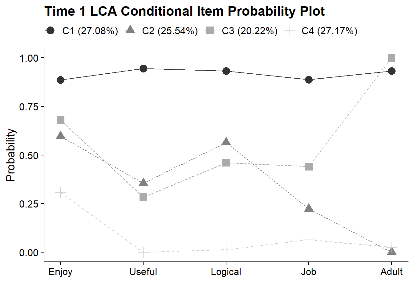
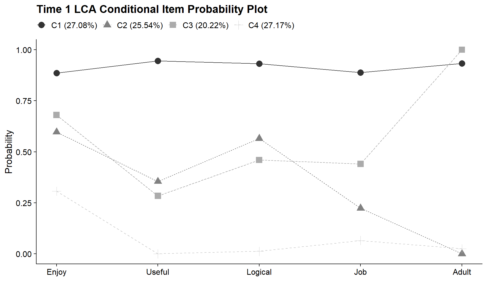
}8.4.2 Time 1 LCA - Conditional Item Probability Plot
plot_lca_function(
  model_name = model_t1_c4,
  item_num = 5,
  class_num = 4,
  item_labels = c("Enjoy","Useful","Logical","Job","Adult"),
  plot_title = "Time 1 LCA Conditional Item Probability Plot"
  )
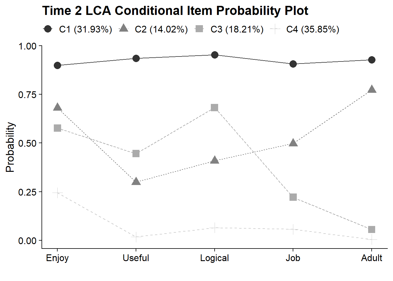
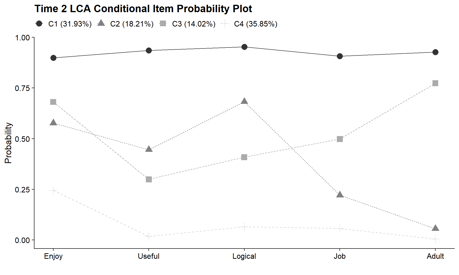
8.4.3 Time 2 LCA - Conditional Item Probability Plot
plot_lca_function(
  model_name = model_t2_c4,
  item_num = 5,
  class_num = 4,
  item_labels = c("Enjoy","Useful","Logical","Job","Adult"),
  plot_title = "Time 2 LCA Conditional Item Probability Plot"
  )
8.5 Estimate Latent Transition Analysis (LTA) Model
8.5.1 Estimate Invariant LTA Model
lta_inv <- mplusObject(

  TITLE =
    "Invariant LTA",

  VARIABLE =
     "usev = ab39m ab39t ab39u ab39w ab39x  ! 7th grade indicators
             ga33a ga33h ga33i ga33k ga33l; ! 10th grade indicators

      categorical = ab39m-ab39x ga33a-ga33l;

      classes = c1(4) c2(4);",

  ANALYSIS =
     "estimator = mlr;
      type = mixture;
      starts = 500 100;
      processors=10;",

  MODEL =
     "%overall%
      c2 on c1;

      MODEL c1:
      %c1#1%
      [AB39M$1-AB39X$1] (1-5);  !!! labels that are repeated will constrain parameters to equality !!!
      %c1#2%
      [AB39M$1-AB39X$1] (6-10);
      %c1#3%
      [AB39M$1-AB39X$1] (11-15);
      %c1#4%
      [AB39M$1-AB39X$1] (16-20);

      MODEL c2:
      %c2#1%
      [GA33A$1-GA33L$1] (1-5);
      %c2#2%
      [GA33A$1-GA33L$1] (6-10);
      %c2#3%
      [GA33A$1-GA33L$1] (11-15);
      %c2#4%
      [GA33A$1-GA33L$1] (16-20);",

  SAVEDATA =
   "file = LTA_Inv_CPROBS.dat;
    save = cprob;
    missflag = 9999;",

  OUTPUT = "tech1 tech15 svalues;",

  usevariables = colnames(lsay_data),
  rdata = lsay_data)

lta_inv_fit <- mplusModeler(lta_inv,
                 dataout=here("lta","lta_model","lta.dat"),
                 modelout=here("lta","lta_model","4-class-invariant.inp"),
                 check=TRUE, run = TRUE, hashfilename = FALSE)
8.5.2 Estimate Non-Invariant Estimated LTA Model
lta_non_inv <- mplusObject(

  TITLE =
    "Non-Invariant LTA",

  VARIABLE =
     "usev = ab39m ab39t ab39u ab39w ab39x  ! 7th grade indicators
             ga33a ga33h ga33i ga33k ga33l; ! 10th grade indicators

      categorical = ab39m-ab39x ga33a-ga33l;

      classes = c1(4) c2(4);",

  ANALYSIS =
     "estimator = mlr;
      type = mixture;
      starts = 500 100;
      processors=10;",

  MODEL =
     "%overall%
      c2 on c1; !!! estimate all multinomial logistic regressions !!!

      !!! The above syntax can also be written as: !!!
               ! c2#1 on c1#1 c1#2 c1#3; !
               ! c2#2 on c1#1 c1#2 c1#3; !
               ! c2#3 on c1#1 c1#2 c1#3; !

      MODEL c1: !!! the following syntax will allow item thresholds to be estimated for each class (e.g. noninvariance) !!!

      %c1#1%
      [AB39M$1-AB39X$1];
      %c1#2%
      [AB39M$1-AB39X$1];
      %c1#3%
      [AB39M$1-AB39X$1];
      %c1#4%
      [AB39M$1-AB39X$1];

      MODEL c2:
      %c2#1%
      [GA33A$1-GA33L$1];
      %c2#2%
      [GA33A$1-GA33L$1];
      %c2#3%
      [GA33A$1-GA33L$1];
      %c2#4%
      [GA33A$1-GA33L$1];",

  OUTPUT = "tech1 tech15 svalues;",

  usevariables = colnames(lsay_data),
  rdata = lsay_data)

lta_non_inv_fit <- mplusModeler(lta_non_inv,
                     dataout=here("lta","lta_model","lta.dat"),
                     modelout=here("lta","lta_model","4-class-non-invariant.inp"),
                     check=TRUE, run = TRUE, hashfilename = FALSE)
8.5.3 Conduct Sattorra-Bentler adjusted Log Likelihood Ratio Difference Testing
non-invariant (comparison): This model has more parameters.
invariant (nested): This model has less parameters.
# *0 = null or nested model & *1 = comparison  or parent model

lta_models <- readModels(here("lta","lta_model"), quiet = TRUE)

# Log Likelihood Values
L0 <- lta_models[["X4.class.invariant.out"]][["summaries"]][["LL"]]
L1 <- lta_models[["X4.class.non.invariant.out"]][["summaries"]][["LL"]]

# LRT equation
lr <- -2*(L0-L1)

# Parameters
p0 <- lta_models[["X4.class.invariant.out"]][["summaries"]][["Parameters"]]
p1 <- lta_models[["X4.class.non.invariant.out"]][["summaries"]][["Parameters"]]

# Scaling Correction Factors
c0 <- lta_models[["X4.class.invariant.out"]][["summaries"]][["LLCorrectionFactor"]]
c1 <- lta_models[["X4.class.non.invariant.out"]][["summaries"]][["LLCorrectionFactor"]]

# Difference Test Scaling correction
cd <- ((p0*c0)-(p1*c1))/(p0-p1)

# Chi-square difference test(TRd)
TRd <- (lr)/(cd)

# Degrees of freedom
df <- abs(p0 - p1)


# Significance test
(p_diff <- pchisq(TRd, df, lower.tail=FALSE))
#> [1] 0.6245173RESULT: The Log Likelihood \(\chi^2\) difference test comparing the invariant and non-invariant LTA models was, \(\chi^2 (20) = 21.542, p = .624\).
Read invariance model and extract parameters (intercepts and multinomial regression coefficients)
lta_inv1 <- readModels(here("lta","lta_model","4-Class-Invariant.out" ), quiet = TRUE)

par <- as_tibble(lta_inv1[["parameters"]][["unstandardized"]]) %>%
  select(1:3) %>%
  filter(grepl('ON|Means', paramHeader)) %>%
  mutate(est = as.numeric(est))
Manual method to calculate transition probabilities:
Although possible to extract transition probabilities directly from the output the following code illustrates how the parameters are used to calculate each transition. This is useful for conducting advanced LTA model specifications such as making specific constraints within or between transition matrices, or testing the equivalence of specific transition probabilities.
# Name each parameter individually to make the subsequent calculations more readable
a1 <- unlist(par[13,3]); a2 <- unlist(par[14,3]); a3 <- unlist(par[15,3]); b11 <- unlist(par[1,3]);
b21 <- unlist(par[4,3]); b31 <- unlist(par[7,3]); b12 <- unlist(par[2,3]); b22 <- unlist(par[5,3]);
b32 <- unlist(par[8,3]); b13 <- unlist(par[3,3]); b23 <- unlist(par[6,3]); b33 <- unlist(par[9,3])

# Calculate transition probabilities from the logit parameters
t11 <- exp(a1+b11)/(exp(a1+b11)+exp(a2+b21)+exp(a3+b31)+exp(0))
t12 <- exp(a2+b21)/(exp(a1+b11)+exp(a2+b21)+exp(a3+b31)+exp(0))
t13 <- exp(a3+b31)/(exp(a1+b11)+exp(a2+b21)+exp(a3+b31)+exp(0))
t14 <- 1 - (t11 + t12 + t13)

t21 <- exp(a1+b12)/(exp(a1+b12)+exp(a2+b22)+exp(a3+b32)+exp(0))
t22 <- exp(a2+b22)/(exp(a1+b12)+exp(a2+b22)+exp(a3+b32)+exp(0))
t23 <- exp(a3+b32)/(exp(a1+b12)+exp(a2+b22)+exp(a3+b32)+exp(0))
t24 <- 1 - (t21 + t22 + t23)

t31 <- exp(a1+b13)/(exp(a1+b13)+exp(a2+b23)+exp(a3+b33)+exp(0))
t32 <- exp(a2+b23)/(exp(a1+b13)+exp(a2+b23)+exp(a3+b33)+exp(0))
t33 <- exp(a3+b33)/(exp(a1+b13)+exp(a2+b23)+exp(a3+b33)+exp(0))
t34 <- 1 - (t31 + t32 + t33)

t41 <- exp(a1)/(exp(a1)+exp(a2)+exp(a3)+exp(0))
t42 <- exp(a2)/(exp(a1)+exp(a2)+exp(a3)+exp(0))
t43 <- exp(a3)/(exp(a1)+exp(a2)+exp(a3)+exp(0))
t44 <- 1 - (t41 + t42 + t43)
8.5.4 Create Transition Table
t_matrix <- tibble(
"Time1" = c("C1=Anti-Science","C1=Amb. w/ Elevated","C1=Amb. w/ Minimal","C1=Pro-Science"),
"C2=Anti-Science" = c(t11,t21,t31,t41),
"C2=Amb. w/ Elevated" = c(t12,t22,t32,t42),
"C2=Amb. w/ Minimal" = c(t13,t23,t33,t43),
"C2=Pro-Science" = c(t14,t24,t34,t44))
t_matrix %>%
gt(rowname_col = "Time1") %>%
tab_stubhead(label = "7th grade") %>%
tab_header(
title = md("**Student transitions from 7th grade (rows) to 10th grade (columns)**"),
subtitle = md(" ")) %>%
fmt_number(2:5,decimals = 2) %>%
tab_spanner(label = "10th grade",columns = 2:5) %>%
tab_footnote(
footnote = md(
"*Note.* Transition matrix values are the identical to Table 5, however Table 5
has the values rearranged by class for interpretation purposes. Classes may be arranged
directly through Mplus syntax using start values."),
locations = cells_title())| Student transitions from 7th grade (rows) to 10th grade (columns)1 | ||||
| 1 | ||||
| 7th grade |
10th grade
|
|||
|---|---|---|---|---|
| C2=Anti-Science | C2=Amb. w/ Elevated | C2=Amb. w/ Minimal | C2=Pro-Science | |
| C1=Anti-Science | 0.27 | 0.27 | 0.32 | 0.15 |
| C1=Amb. w/ Elevated | 0.09 | 0.56 | 0.19 | 0.16 |
| C1=Amb. w/ Minimal | 0.15 | 0.21 | 0.52 | 0.12 |
| C1=Pro-Science | 0.08 | 0.35 | 0.27 | 0.30 |
| 1 Note. Transition matrix values are the identical to Table 5, however Table 5 has the values rearranged by class for interpretation purposes. Classes may be arranged directly through Mplus syntax using start values. | ||||
8.6 Adding Covariates
We use the ML three-step method to estimate LTA models with predictors and distal outcomes). Estimate the unconditional model for each latent variable with the predictors included in the auxiliary option for at least one of the models.
Covariates
-
sci_issues7: Interest in science issues (1 = Not at all interested, 2 = Moderately Interested, 3 = Very interested)
-
sci_irt7: 7th Grade Science IRT Score (Continuous)
-
female: Gender (0 = Male, 1 = Female)
8.6.1 Step 1 - Estimate Unconditional Model w/ Auxiliary Specification
7th Grade
step1  <- mplusObject(
  TITLE = "Step 1 - T1",
  VARIABLE =
  "usevar = ab39m ab39t ab39u ab39w ab39x;
  categorical = ab39m ab39t ab39u ab39w ab39x;

   classes = c(4);

   auxiliary = sci_issues7 sci_irt7 female;

   idvariable = casenum;",

  ANALYSIS =
   "estimator = mlr;
    type = mixture;
    starts = 0;
    optseed = 534483;",

  SAVEDATA =
   "File=3step_t1.dat;
    Save=cprob;",

  OUTPUT = "residual tech11 tech14 svalues",

  PLOT =
    "type = plot3;
    series = ab39m-ab39x(*);",

  usevariables = colnames(lsay_data),
  rdata = lsay_data)

step1_fit <- mplusModeler(step1,
                            dataout=here("lta","cov_model","t1.dat"),
                            modelout=here("lta","cov_model","one_T1.inp") ,
                            check=TRUE, run = TRUE, hashfilename = FALSE)
10th Grade
step1  <- mplusObject(
  TITLE = "Step 1 - T1",
  VARIABLE =
  "usevar =  ga33a ga33h ga33i ga33k ga33l;
  categorical =  ga33a ga33h ga33i ga33k ga33l;

   classes = c(4);

   !auxiliary = sci_issues7 sci_irt7 female;

   idvariable = casenum;",

  ANALYSIS =
   "estimator = mlr;
    type = mixture;
    starts = 0;
    optseed = 392418;",

  SAVEDATA =
   "File=3step_t2.dat;
    Save=cprob;",

  OUTPUT = "residual tech11 tech14 svalues",

  PLOT =
    "type = plot3;
    series = ga33a-ga33l(*);",

  usevariables = colnames(lsay_data),
  rdata = lsay_data)

step1_fit <- mplusModeler(step1,
                            dataout=here("lta","cov_model","t2.dat"),
                            modelout=here("lta","cov_model","one_T2.inp") ,
                            check=TRUE, run = TRUE, hashfilename = FALSE)
Plot Time 1
output_T1 <- readModels(here("lta","cov_model","one_T1.out"))

plot_lca_function(
  model_name = output_T1,
  item_num = 5,
  class_num = 4,
  item_labels = c("Enjoy","Useful","Logical","Job","Adult"),
  plot_title = "Time 1 LCA Conditional Item Probability Plot"
  )
Plot Time 2
output_T2 <- readModels(here("lta","cov_model","one_T2.out"))

plot_lca_function(
  model_name = output_T2,
  item_num = 5,
  class_num = 4,
  item_labels = c("Enjoy","Useful","Logical","Job","Adult"),
  plot_title = "Time 2 LCA Conditional Item Probability Plot"
  )
8.6.2 Step 2 - Determine Measurement Error
Extract logits for the classification probabilities for the most likely latent class:
logit_cprobs_T1 <- as.data.frame(output_T1[["class_counts"]]
                                       [["logitProbs.mostLikely"]])

logit_cprobs_T2 <- as.data.frame(output_T2[["class_counts"]]
                                       [["logitProbs.mostLikely"]])
Extract saved dataset:
savedata_T1 <- as.data.frame(output_T1[["savedata"]])
savedata_T2 <- as.data.frame(output_T2[["savedata"]])
Rename the column in savedata named “C” and change to “N”
colnames(savedata_T1)[colnames(savedata_T1)=="C"] <- "N_T1"
colnames(savedata_T2)[colnames(savedata_T2)=="C"] <- "N_T2"

savedata <- savedata_T1 %>%
  full_join(savedata_T2, by = "CASENUM")
8.6.3 Step 3 - Add Auxiliary Variables
step3  <- mplusObject(
  TITLE = "ML Three Step LTA Model",

  VARIABLE =
 "nominal=N_T1 N_T2;
  usevar = N_T1 N_T2 SCI_IRT7 FEMALE;
  classes = c1(4) c2(4);" ,

  ANALYSIS =
 "estimator = mlr;
  type = mixture;
  starts = 0;",

  MODEL =
  glue(
 " %OVERALL%

   c2 on c1;
   c1 c2 on  SCI_IRT7 FEMALE;

  MODEL c1:

  %c1#1%
  [N_T1#1@{logit_cprobs_T1[1,1]}];
  [N_T1#2@{logit_cprobs_T1[1,2]}];
  [N_T1#3@{logit_cprobs_T1[1,3]}];

  %c1#2%
  [N_T1#1@{logit_cprobs_T1[2,1]}];
  [N_T1#2@{logit_cprobs_T1[2,2]}];
  [N_T1#3@{logit_cprobs_T1[2,3]}];

  %c1#3%
  [N_T1#1@{logit_cprobs_T1[3,1]}];
  [N_T1#2@{logit_cprobs_T1[3,2]}];
  [N_T1#3@{logit_cprobs_T1[3,3]}];

  %c1#4%
  [N_T1#1@{logit_cprobs_T1[4,1]}];
  [N_T1#2@{logit_cprobs_T1[4,2]}];
  [N_T1#3@{logit_cprobs_T1[4,3]}];


  MODEL c2:

  %c2#1%
  [N_T2#1@{logit_cprobs_T2[1,1]}];
  [N_T2#2@{logit_cprobs_T2[1,2]}];
  [N_T2#3@{logit_cprobs_T2[1,3]}];

  %c2#2%
  [N_T2#1@{logit_cprobs_T2[2,1]}];
  [N_T2#2@{logit_cprobs_T2[2,2]}];
  [N_T2#3@{logit_cprobs_T2[2,3]}];


  %c2#3%
  [N_T2#1@{logit_cprobs_T2[3,1]}];
  [N_T2#2@{logit_cprobs_T2[3,2]}];
  [N_T2#3@{logit_cprobs_T2[3,3]}];

   %c2#4%
  [N_T2#1@{logit_cprobs_T2[4,1]}];
  [N_T2#2@{logit_cprobs_T2[4,2]}];
  [N_T2#3@{logit_cprobs_T2[4,3]}];"),


  OUTPUT = "tech15;",

  usevariables = colnames(savedata),
  rdata = savedata)

step3_fit <- mplusModeler(step3,
               dataout=here("lta","cov_model","three.dat"),
               modelout=here("lta","cov_model","three.inp"),
               check=TRUE, run = TRUE, hashfilename = FALSE)
8.6.3.1 LTA Transition Plot
This code is adapted from the source code for the plotLTA function found in the
NOTE: The function found in plot_transitions_function.R is specific to a model with 2 time-points and 4-classes & must be updated to accommodate other models.
source(here("functions","plot_transitions_function.R"))

lta_model <- readModels(here("lta","cov_model","three.out"))

plot_transitions_function(
  model_name = lta_model,
  color_pallete = pnw_palette("Bay", n=4, type = "discrete"),
  facet_labels =c(
    `1` = "Transitions to 10th Grade from the Pro-Science w/ Elevated Utility Class",
    `2` = "Transitions to 10th Grade from the Ambivalent w/ Elevated Utility Class",
    `3` = "Transitions to 10th Grade from the Ambivalent w/ Minimal Utility Class",
    `4` = "Transitions to 10th Grade from the Anti-Science w/ Minimal Utility Class"),
  timepoint_labels = c('1' = "7th Grade", '2' = "10th Grade"),
  class_labels = c(
    "Pro-Science",
    "Amb. / Elev. Utility",
    "Amb. / Min. Utility",
    "Anti-Science")
  )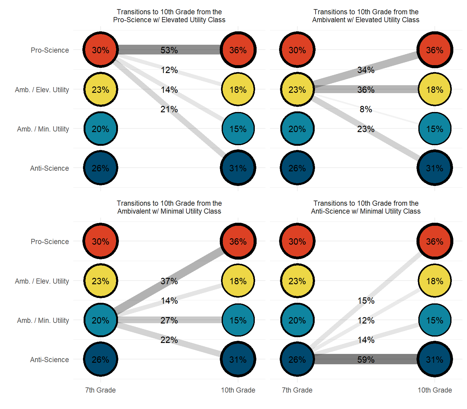
Table:
lta_prob <- as.data.frame(lta_model$class_counts$transitionProbs$probability)


t_matrix <- tibble(
  "7th Grade" = c("Pro-Science","Amb. / Elev. Utility","Amb. / Min. Utility","Anti-Science"),
  "Pro-Science" = c(lta_prob[1,1],lta_prob[2,1],lta_prob[3,1],lta_prob[4,1]),
  "Amb. / Elev. Utility" = c(lta_prob[5,1],lta_prob[6,1],lta_prob[7,1],lta_prob[8,1]),
  "Amb. / Min. Utility" = c(lta_prob[9,1],lta_prob[10,1],lta_prob[11,1],lta_prob[12,1]),
  "Anti-Science" = c(lta_prob[13,1],lta_prob[14,1],lta_prob[15,1],lta_prob[16,1]))

t_matrix %>%
  gt(rowname_col = "7th Grade") %>%
  tab_stubhead(label = "7th Grade") %>%
  tab_header(
    title = md("**Transition Probabilities**")) %>%
  fmt_number(2:5,decimals = 2) %>%
tab_spanner(label = "10th Grade",columns = 2:5)#%>% | Transition Probabilities | ||||
| 7th Grade |
10th Grade
|
|||
|---|---|---|---|---|
| Pro-Science | Amb. / Elev. Utility | Amb. / Min. Utility | Anti-Science | |
| Pro-Science | 0.53 | 0.12 | 0.14 | 0.21 |
| Amb. / Elev. Utility | 0.34 | 0.35 | 0.08 | 0.23 |
| Amb. / Min. Utility | 0.37 | 0.14 | 0.27 | 0.22 |
| Anti-Science | 0.15 | 0.12 | 0.14 | 0.59 |
#gtsave("matrix.docx")8.6.3.2 Covariate Table
# REFERENCE CLASS 4
cov <- as.data.frame(lta_model[["parameters"]][["unstandardized"]]) %>%
  filter(param %in% c("SCI_IRT7", "FEMALE")) %>%
  mutate(param = case_when(
            param == "SCI_IRT7" ~ "Science IRT Score",
            param == "FEMALE" ~ "Gender"),
    se = paste0("(", format(round(se,2), nsmall =2), ")")) %>%
  separate(paramHeader, into = c("Time", "Class"), sep = "#") %>%
  mutate(Class = case_when(
            Class == "1.ON" ~ "Pro-Science",
            Class == "2.ON" ~ "Amb. / Elev. Utility",
            Class == "3.ON" ~ "Amb. / Min. Utility"),
         Time = case_when(
            Time == "C1" ~ "7th Grade (T1)",
            Time == "C2" ~ "10th Grade (T2)",
         )
         ) %>%
  unite(estimate, est, se, sep = " ") %>%
  select(Time:pval, -est_se) %>%
  mutate(pval = ifelse(pval<0.001, paste0("<.001*"),
                       ifelse(pval<0.05, paste0(scales::number(pval, accuracy = .001), "*"),
                              scales::number(pval, accuracy = .001))))


# Create table

cov_m1 <- cov %>%
  group_by(param, Class) %>%
  gt() %>%
  tab_header(
    title = "Relations Between the Covariates and Latent Class") %>%
  tab_footnote(
    footnote = md(
      "Reference Group: Anti-Science"
    ),
locations = cells_title()
  ) %>%
  cols_label(
    param = md("Covariate"),
    estimate = md("Estimate (*se*)"),
    pval = md("*p*-value")) %>%
  sub_missing(1:3,
              missing_text = "") %>%
  sub_values(values = c(999.000), replacement = "-") %>%
  cols_align(align = "center") %>%
  opt_align_table_header(align = "left") %>%
  gt::tab_options(table.font.names = "serif")

cov_m1| Relations Between the Covariates and Latent Class1 | ||
| Time | Estimate (se) | p-value |
|---|---|---|
| Science IRT Score - Pro-Science | ||
| 7th Grade (T1) | 0.05 (0.01) | <.001* |
| 10th Grade (T2) | 0.056 (0.01) | <.001* |
| Gender - Pro-Science | ||
| 7th Grade (T1) | -1.001 (0.23) | <.001* |
| 10th Grade (T2) | 0.011 (0.22) | 0.962 |
| Science IRT Score - Amb. / Elev. Utility | ||
| 7th Grade (T1) | -0.012 (0.01) | 0.351 |
| 10th Grade (T2) | 0.049 (0.02) | 0.002* |
| Gender - Amb. / Elev. Utility | ||
| 7th Grade (T1) | -0.515 (0.28) | 0.071 |
| 10th Grade (T2) | -0.111 (0.33) | 0.737 |
| Science IRT Score - Amb. / Min. Utility | ||
| 7th Grade (T1) | 0.021 (0.01) | 0.093 |
| 10th Grade (T2) | 0.022 (0.02) | 0.202 |
| Gender - Amb. / Min. Utility | ||
| 7th Grade (T1) | -0.761 (0.26) | 0.003* |
| 10th Grade (T2) | 0.075 (0.32) | 0.815 |
| 1 Reference Group: Anti-Science | ||
8.6.3.3 Manually calculate transition probabilities by covariate
step3  <- mplusObject(
  TITLE = "LTA (invariant)",

  VARIABLE =
 "usevar = ab39m ab39t ab39u ab39w ab39x  ! 7th grade indicators
               ga33a ga33h ga33i ga33k ga33l FEMALE;
  categorical = ab39m-ab39x ga33a-ga33l;
  classes = c1(4) c2(4);" ,

  ANALYSIS =
 "estimator = mlr;
  type = mixture;
  starts = 500 100;
 processors = 10;",

  MODEL =
  "%overall%

    c2 c1 on FEMALE;

      c2#1 on c1#1 (b11);
      c2#2 on c1#1 (b21);
      c2#3 on c1#1 (b31);

      c2#1 on c1#2 (b12);
      c2#2 on c1#2 (b22);
      c2#3 on c1#2 (b32);

      c2#1 on c1#3 (b13);
      c2#2 on c1#3 (b23);
      c2#3 on c1#3 (b33);

      [c2#1] (a1);
      [c2#2] (a2);
      [c2#3] (a3);

     c2#1 ON female (b212);
     c2#2 ON female (b222);
     c2#3 ON female (b232);
     c1#1 ON female (b112);
     c1#2 ON female (b122);
     c1#3 ON female (b132);

      MODEL c1:
      %c1#1%
      [AB39M$1-AB39X$1] (1-5);  !!! labels that are repeated will constrain parameters to equality !!!
      %c1#2%
      [AB39M$1-AB39X$1] (6-10);
      %c1#3%
      [AB39M$1-AB39X$1] (11-15);
      %c1#4%
      [AB39M$1-AB39X$1] (16-20);

      MODEL c2:
      %c2#1%
      [GA33A$1-GA33L$1] (1-5);
      %c2#2%
      [GA33A$1-GA33L$1] (6-10);
      %c2#3%
      [GA33A$1-GA33L$1] (11-15);
      %c2#4%
      [GA33A$1-GA33L$1] (16-20);",


  OUTPUT = "tech1 tech15 svalues;",

  MODELCONSTRAINT = "  ! Compute joint and marginal probabilities:
        New(
        t11 t12 t13 t14
        t21 t22 t23 t24
        t31 t32 t33 t34
        t41 t42 t43 t44

        t11B t12B t13B t14B
        t21B t22B t23B t24B
        t31B t32B t33B t34B
        t41B t42B t43B t44B

        diff_11_22 x

       );

        t11 = exp(a1 +b11)/(exp(a1+b11)+exp(a2+b21)+exp(a3+b31)+exp(0));
        t12 = exp(a2 +b21)/(exp(a1+b11)+exp(a2+b21)+exp(a3+b31)+exp(0));
        t13 = exp(a3 +b31)/(exp(a1+b11)+exp(a2+b21)+exp(a3+b31)+exp(0));
        t14 = 1 - (t11+t12+t13);

        t21 = exp(a1 +b12)/(exp(a1+b12)+exp(a2+b22)+exp(a3+b32)+exp(0));
        t22 = exp(a2 +b22)/(exp(a1+b12)+exp(a2+b22)+exp(a3+b32)+exp(0));
        t23 = exp(a3 +b32)/(exp(a1+b12)+exp(a2+b22)+exp(a3+b32)+exp(0));
        t24 = 1 - (t21+t22+t23);

        t31 = exp(a1 +b13)/(exp(a1+b13)+exp(a2+b23)+exp(a3+b33)+exp(0));
        t32 = exp(a2 +b23)/(exp(a1+b13)+exp(a2+b23)+exp(a3+b33)+exp(0));
        t33 = exp(a3 +b33)/(exp(a1+b13)+exp(a2+b23)+exp(a3+b33)+exp(0));
        t34 = 1 - (t31+t32+t33);

        t41 = exp(a1)/(exp(a1)+exp(a2)+exp(a3)+exp(0));
        t42 = exp(a2)/(exp(a1)+exp(a2)+exp(a3)+exp(0));
        t43 = exp(a3)/(exp(a1)+exp(a2)+exp(a3)+exp(0));
        t44 = 1 - (t41+t42+t43);


     !c1#3 ON female (b132);

 x= 1  ; ! x=1 is female, x=0 males

t11B = exp(a1 +b11+b212*x)/(exp(a1+b11+b212*x)+exp(a2+b21+b222*x)+exp(a3+b31+b232*x)
+exp(0));
t12B = exp(a2 +b21+b222*x)/(exp(a1+b11+b212*x)+exp(a2+b21+b222*x)+exp(a3+b31+b232*x)
+exp(0));
t13B = exp(a3 +b31+b232*x)/(exp(a1+b11+b212*x)+exp(a2+b21+b222*x)+exp(a3+b31+b232*x)
+exp(0));
t14B = 1 - (t11B+t12B+t13B);

t21B = exp(a1 +b12+b212*x)/(exp(a1+b12+b212*x)+exp(a2+b22+b222*x)+exp(a3+b32+b232*x)
+exp(0));
t22B = exp(a2 +b22+b222*x)/(exp(a1+b12+b212*x)+exp(a2+b22+b222*x)+exp(a3+b32+b232*x)
+exp(0));
t23B = exp(a3 +b32+b232*x)/(exp(a1+b12+b212*x)+exp(a2+b22+b222*x)+exp(a3+b32+b232*x)
+exp(0));
t24B = 1 - (t21B+t22B+t23B);

t31B = exp(a1 +b13+b212*x)/(exp(a1+b13+b212*x)+exp(a2+b23+b222*x)+exp(a3+b33+b232*x)
+exp(0));
t32B = exp(a2 +b23+b222*x)/(exp(a1+b13+b212*x)+exp(a2+b23+b222*x)+exp(a3+b33+b232*x)
+exp(0));
t33B = exp(a3 +b33+b232*x)/(exp(a1+b13+b212*x)+exp(a2+b23+b222*x)+exp(a3+b33+b232*x)
+exp(0));
t34B = 1 - (t31B+t32B+t33B);

t41B = exp(a1+b212*x)/(exp(a1+b212*x)+exp(a2+b222*x)+exp(a3+b232*x)+exp(0));
t42B = exp(a2+b222*x)/(exp(a1+b212*x)+exp(a2+b222*x)+exp(a3+b232*x)+exp(0));
t43B = exp(a3+b232*x)/(exp(a1+b212*x)+exp(a2+b222*x)+exp(a3+b232*x)+exp(0));
t44B = 1 - (t41B+t42B+t43B);

        diff_11_22= t11-t11B;",

  usevariables = colnames(savedata),
  rdata = savedata)

step3_fit <- mplusModeler(step3,
               dataout=here("lta","cov_model","calc_tran.dat"),
               modelout=here("lta","cov_model","calc_tran.inp"),
               check=TRUE, run = TRUE, hashfilename = FALSE)
Read invariance model and extract parameters (intercepts and multinomial regression coefficients)
lta_inv1 <- readModels(here("lta","cov_model","calc_tran.out" ), quiet = TRUE)

par <- as_tibble(lta_inv1[["parameters"]][["unstandardized"]]) %>%
  select(1:3) %>%
  filter(grepl('ON|Means|Intercept', paramHeader)) %>%
  mutate(est = as.numeric(est),
         label = c("b11", "b12", "b13", "b21", "b22", "b23", "b31", "b32", "b33", "b212", "b222", "b232", "b112", "b122", "b132", "a11", "a21", "a31", "a12", "a22", "a32"))
Manual method to calculate transition probabilities by covariate:
# Name each parameter individually to make the subsequent calculations more readable
a1 <- unlist(par[19,3]);
a2 <- unlist(par[20,3]);
a3 <- unlist(par[21,3]);

b11 <- unlist(par[1,3]);
b21 <- unlist(par[4,3]);
b31 <- unlist(par[7,3]);

b12 <- unlist(par[2,3]);
b22 <- unlist(par[5,3]);
b32 <- unlist(par[8,3]);

b13 <- unlist(par[3,3]);
b23 <- unlist(par[6,3]);
b33 <- unlist(par[9,3]);

b212 <- unlist(par[10,3]);
b222 <- unlist(par[11,3]);
b232 <- unlist(par[12,3]);

b112 <- unlist(par[13,3]);
b122 <- unlist(par[14,3]);
b132 <- unlist(par[15,3]);

x <- 0 # x=1 is female, x=0 males

# Calculate transition probabilities from the logit parameters
t11B <- exp(a1 + b11 + b212*x) / (exp(a1 + b11 + b212*x) + exp(a2 + b21 + b222*x) + exp(a3 + b31 + b232*x) + exp(0))
t12B <- exp(a2 + b21 + b222*x) / (exp(a1 + b11 + b212*x) + exp(a2 + b21 + b222*x) + exp(a3 + b31 + b232*x) + exp(0))
t13B <- exp(a3 + b31 + b232*x) / (exp(a1 + b11 + b212*x) + exp(a2 + b21 + b222*x) + exp(a3 + b31 + b232*x) + exp(0))
t14B <- 1 - (t11B + t12B + t13B)

t21B <- exp(a1 + b12 + b212*x) / (exp(a1 + b12 + b212*x) + exp(a2 + b22 + b222*x) + exp(a3 + b32 + b232*x) + exp(0))
t22B <- exp(a2 + b22 + b222*x) / (exp(a1 + b12 + b212*x) + exp(a2 + b22 + b222*x) + exp(a3 + b32 + b232*x) + exp(0))
t23B <- exp(a3 + b32 + b232*x) / (exp(a1 + b12 + b212*x) + exp(a2 + b22 + b222*x) + exp(a3 + b32 + b232*x) + exp(0))
t24B <- 1 - (t21B + t22B + t23B)

t31B <- exp(a1 + b13 + b212*x) / (exp(a1 + b13 + b212*x) + exp(a2 + b23 + b222*x) + exp(a3 + b33 + b232*x) + exp(0))
t32B <- exp(a2 + b23 + b222*x) / (exp(a1 + b13 + b212*x) + exp(a2 + b23 + b222*x) + exp(a3 + b33 + b232*x) + exp(0))
t33B <- exp(a3 + b33 + b232*x) / (exp(a1 + b13 + b212*x) + exp(a2 + b23 + b222*x) + exp(a3 + b33 + b232*x) + exp(0))
t34B <- 1 - (t31B + t32B + t33B)

t41B <- exp(a1 + b212*x) / (exp(a1 + b212*x) + exp(a2 + b222*x) + exp(a3 + b232*x) + exp(0))
t42B <- exp(a2 + b222*x) / (exp(a1 + b212*x) + exp(a2 + b222*x) + exp(a3 + b232*x) + exp(0))
t43B <- exp(a3 + b232*x) / (exp(a1 + b212*x) + exp(a2 + b222*x) + exp(a3 + b232*x) + exp(0))
t44B <- 1 - (t41B + t42B + t43B)

x <- 1 # x=1 is female, x=0 males

# Calculate transition probabilities from the logit parameters
t11 <- exp(a1 + b11 + b212*x) / (exp(a1 + b11 + b212*x) + exp(a2 + b21 + b222*x) + exp(a3 + b31 + b232*x) + exp(0))
t12 <- exp(a2 + b21 + b222*x) / (exp(a1 + b11 + b212*x) + exp(a2 + b21 + b222*x) + exp(a3 + b31 + b232*x) + exp(0))
t13 <- exp(a3 + b31 + b232*x) / (exp(a1 + b11 + b212*x) + exp(a2 + b21 + b222*x) + exp(a3 + b31 + b232*x) + exp(0))
t14 <- 1 - (t11 + t12 + t13)

t21 <- exp(a1 + b12 + b212*x) / (exp(a1 + b12 + b212*x) + exp(a2 + b22 + b222*x) + exp(a3 + b32 + b232*x) + exp(0))
t22 <- exp(a2 + b22 + b222*x) / (exp(a1 + b12 + b212*x) + exp(a2 + b22 + b222*x) + exp(a3 + b32 + b232*x) + exp(0))
t23 <- exp(a3 + b32 + b232*x) / (exp(a1 + b12 + b212*x) + exp(a2 + b22 + b222*x) + exp(a3 + b32 + b232*x) + exp(0))
t24 <- 1 - (t21 + t22 + t23)

t31 <- exp(a1 + b13 + b212*x) / (exp(a1 + b13 + b212*x) + exp(a2 + b23 + b222*x) + exp(a3 + b33 + b232*x) + exp(0))
t32 <- exp(a2 + b23 + b222*x) / (exp(a1 + b13 + b212*x) + exp(a2 + b23 + b222*x) + exp(a3 + b33 + b232*x) + exp(0))
t33 <- exp(a3 + b33 + b232*x) / (exp(a1 + b13 + b212*x) + exp(a2 + b23 + b222*x) + exp(a3 + b33 + b232*x) + exp(0))
t34 <- 1 - (t31 + t32 + t33)

t41 <- exp(a1 + b212*x) / (exp(a1 + b212*x) + exp(a2 + b222*x) + exp(a3 + b232*x) + exp(0))
t42 <- exp(a2 + b222*x) / (exp(a1 + b212*x) + exp(a2 + b222*x) + exp(a3 + b232*x) + exp(0))
t43 <- exp(a3 + b232*x) / (exp(a1 + b212*x) + exp(a2 + b222*x) + exp(a3 + b232*x) + exp(0))
t44 <- 1 - (t41 + t42 + t43)
Create table
8.6.4 Create Transition Table
t_matrix <- tibble(
  "Time1" = c("C1=Anti-Science","C1=Amb. w/ Elevated","C1=Amb. w/ Minimal","C1=Pro-Science"),
  "C2=Anti-Science" = c(t11,t21,t31,t41),
  "C2=Amb. w/ Elevated" = c(t12,t22,t32,t42),
  "C2=Amb. w/ Minimal" = c(t13,t23,t33,t43),
  "C2=Pro-Science" = c(t14,t24,t34,t44))

t_matrix %>%
  gt(rowname_col = "Time1") %>%
  tab_stubhead(label = "7th grade") %>%
  tab_header(
    title = md("**FEMALES: Student transitions from 7th grade (rows) to 10th grade (columns)**")) %>%
  fmt_number(2:5,decimals = 3) %>%
  tab_spanner(label = "10th grade",columns = 2:5) %>%
  tab_footnote(
    footnote = md(
    "*Note.* Transition matrix values are the identical to Table 5, however Table 5
    has the values rearranged by class for interpretation purposes. Classes may be arranged
    directly through Mplus syntax using start values."),
locations = cells_title())| FEMALES: Student transitions from 7th grade (rows) to 10th grade (columns)1 | ||||
| 7th grade |
10th grade
|
|||
|---|---|---|---|---|
| C2=Anti-Science | C2=Amb. w/ Elevated | C2=Amb. w/ Minimal | C2=Pro-Science | |
| C1=Anti-Science | 0.302 | 0.261 | 0.097 | 0.341 |
| C1=Amb. w/ Elevated | 0.129 | 0.510 | 0.152 | 0.209 |
| C1=Amb. w/ Minimal | 0.164 | 0.308 | 0.273 | 0.255 |
| C1=Pro-Science | 0.177 | 0.187 | 0.094 | 0.542 |
| 1 Note. Transition matrix values are the identical to Table 5, however Table 5 has the values rearranged by class for interpretation purposes. Classes may be arranged directly through Mplus syntax using start values. | ||||
t_matrix <- tibble(
  "Time1" = c("C1=Anti-Science","C1=Amb. w/ Elevated","C1=Amb. w/ Minimal","C1=Pro-Science"),
  "C2=Anti-Science" = c(t11B,t21B,t31B,t41B),
  "C2=Amb. w/ Elevated" = c(t12B,t22B,t32B,t42B),
  "C2=Amb. w/ Minimal" = c(t13B,t23B,t33B,t43B),
  "C2=Pro-Science" = c(t14B,t24B,t34B,t44B))

t_matrix %>%
  gt(rowname_col = "Time1") %>%
  tab_stubhead(label = "7th grade") %>%
  tab_header(
    title = md("**MALES: Student transitions from 7th grade (rows) to 10th grade (columns)**")) %>%
  fmt_number(2:5,decimals = 3) %>%
  tab_spanner(label = "10th grade",columns = 2:5) %>%
  tab_footnote(
    footnote = md(
    "*Note.* Transition matrix values are the identical to Table 5, however Table 5
    has the values rearranged by class for interpretation purposes. Classes may be arranged
    directly through Mplus syntax using start values."),
locations = cells_title())| MALES: Student transitions from 7th grade (rows) to 10th grade (columns)1 | ||||
| 7th grade |
10th grade
|
|||
|---|---|---|---|---|
| C2=Anti-Science | C2=Amb. w/ Elevated | C2=Amb. w/ Minimal | C2=Pro-Science | |
| C1=Anti-Science | 0.306 | 0.273 | 0.085 | 0.336 |
| C1=Amb. w/ Elevated | 0.131 | 0.532 | 0.133 | 0.205 |
| C1=Amb. w/ Minimal | 0.170 | 0.329 | 0.245 | 0.256 |
| C1=Pro-Science | 0.181 | 0.198 | 0.083 | 0.539 |
| 1 Note. Transition matrix values are the identical to Table 5, however Table 5 has the values rearranged by class for interpretation purposes. Classes may be arranged directly through Mplus syntax using start values. | ||||