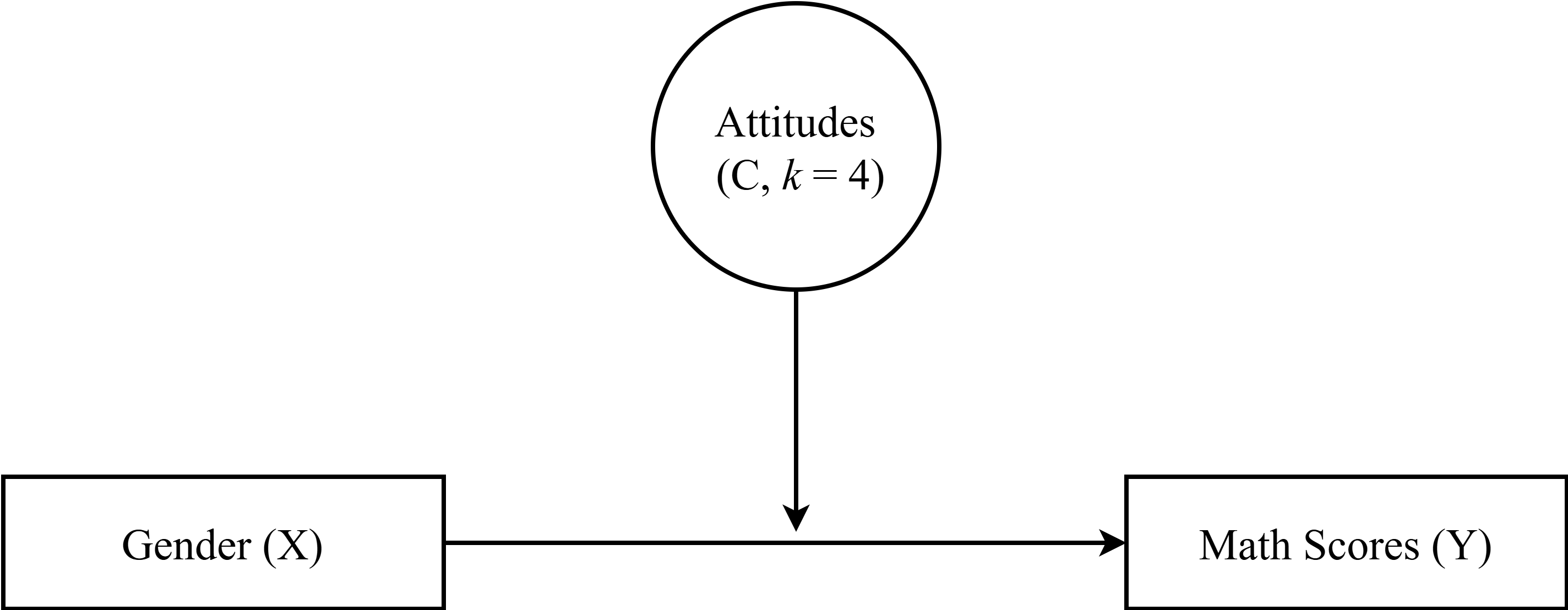
7 LCA Moderation
Example: Longitudinal Study of American Youth
Data source: : See documentation here
7.1 Load Packages
library(MplusAutomation)
library(tidyverse)
library(here)
library(glue)
library(gt)
library(cowplot)
library(kableExtra)
library(psych)
library(float)
library(janitor)
7.2 Moderation Path Diagram
| LCA Indicators & Auxiliary Variables: Math Attitudes Example | |
| Name | Variable Description |
|---|---|
| enjoy | I enjoy math. |
| useful | Math is useful in everyday problems. |
| logical | Math helps a person think logically. |
| job | It is important to know math to get a good job. |
| adult | I will use math in many ways as an adult. |
| Auxiliary Variables | |
| female | Self-reported student gender (0=Male, 1=Female). |
| math_irt | Standardized IRT math test score - 12th grade. |
Read in LSAY dataset
data <- read_csv(here("data","lsay_subset.csv")) %>%
  clean_names() %>%   # make variable names lowercase
  mutate(female = recode(gender, `1` = 0, `2` = 1)) # relabel values from 1,2 to 0,1
7.3 Descriptive Statistics
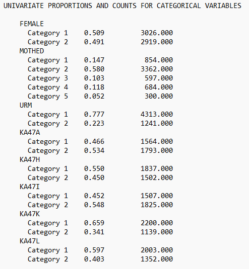
7.3.1 Descriptive Statistics using R:
Quick view of all the relevant variables:
Proportion of indicators using R:
# Set up data to find proportions of binary indicators
ds <- data %>%
  pivot_longer(c(enjoy, useful, logical, job, adult), names_to = "Variable")

# Create table of variables and counts
tab <- table(ds$Variable, ds$value)

# Find proportions and round to 3 decimal places
prop <- prop.table(tab, margin = 1) %>%
  round(3)

# Combine everything to one table
dframe <- data.frame(Variables=rownames(tab), Proportion=prop[,2], Count=tab[,2])
#remove row names
row.names(dframe) <- NULL
gt(dframe) %>%
tab_header(title = md("**LCA Indicator Proportions**"), subtitle = md(" ")) %>%
tab_options(column_labels.font.weight = "bold", row_group.font.weight = "bold") | LCA Indicator Proportions | ||
| Variables | Proportion | Count |
|---|---|---|
| adult | 0.702 | 1858 |
| enjoy | 0.669 | 1784 |
| job | 0.743 | 1947 |
| logical | 0.640 | 1686 |
| useful | 0.695 | 1835 |
7.3.2 Descriptive Statistics using MplusAutomation:
basic_mplus  <- mplusObject(
  TITLE = "LSAL Descriptive Statistics;",

  VARIABLE =
    "usevar = enjoy, useful, logical, job, adult, female, math_irt;
    categorical = enjoy, useful, logical, job, adult, female;",

  ANALYSIS = "TYPE=basic;",

  OUTPUT = "sampstat;",

  usevariables = colnames(data),
  rdata = data)

basic_mplus_fit <- mplusModeler(basic_mplus,
                            dataout = here("moderation", "LSAL_data.dat"),
                            modelout = here("moderation","basic.inp"),
                            check = TRUE, run = TRUE, hashfilename = FALSE)
View the .out file:
Or, view of descriptive statistics using get_sampstat():
# Using MplusAutomation
MplusAutomation::get_sampstat(basic_mplus_fit)

# Using base R
summary(data)
7.4 Enumeration
This code uses the mplusObject function in the MplusAutomation package and saves all model runs in the mplus_enum folder.
lca_enum_6  <- lapply(1:6, function(k) {
  lca_enum  <- mplusObject(

    TITLE = glue("{k}-Class"),

    VARIABLE = glue(
      "categorical = enjoy, useful, logical, job, adult;
     usevar = enjoy, useful, logical, job, adult;
     classes = c({k});"),

    ANALYSIS =
      "estimator = mlr;
    type = mixture;
    processors = 12;
    starts = 500 100;",

    OUTPUT = "sampstat residual tech11 tech14;",

    usevariables = colnames(data),
    rdata = data)

  lca_enum_fit <- mplusModeler(lca_enum,
                               dataout=glue(here("moderation","enum", "LSAY_data.dat")),
                               modelout=glue(here("moderation","enum", "c{k}_lsal.inp")) ,
                               check=TRUE, run = TRUE, hashfilename = FALSE)
})IMPORTANT: Before moving forward, make sure to examine each output document to ensure models were estimated normally. In this example, the last model (6-class models) did not produce reliable output and was excluded.
7.4.1 Table of Fit
First, extract data:
source(here("functions", "extract_mplus_info.R"))

# Define the directory where all of the .out files are located.
output_dir <- here("moderation","enum")

# Get all .out files
output_files <- list.files(output_dir, pattern = "\\.out$", full.names = TRUE)

# Process all .out files into one dataframe
final_data <- map_dfr(output_files, extract_mplus_info_extended)

# Extract Sample_Size from final_data
sample_size <- unique(final_data$Sample_Size)
7.4.1.1 Examine Mplus Warnings
source(here("functions", "extract_warnings.R"))

warnings_table <- extract_warnings(final_data)
warnings_table| Model Warnings | ||
| Output File | # of Warnings | Warning Message(s) |
|---|---|---|
| c1_lsal.out | There are 4 warnings in the output file. | *** WARNING in OUTPUT command SAMPSTAT option is not available when all outcomes are censored, ordered categorical, unordered categorical (nominal), count or continuous-time survival variables. Request for SAMPSTAT is ignored. |
*** WARNING in OUTPUT command TECH11 option is not available for TYPE=MIXTURE with only one class. Request for TECH11 is ignored. |
||
*** WARNING in OUTPUT command TECH14 option is not available for TYPE=MIXTURE with only one class. Request for TECH14 is ignored. |
||
*** WARNING Data set contains cases with missing on all variables. These cases were not included in the analysis. Number of cases with missing on all variables: 441 |
||
| c2_lsal.out | There are 2 warnings in the output file. | *** WARNING in OUTPUT command SAMPSTAT option is not available when all outcomes are censored, ordered categorical, unordered categorical (nominal), count or continuous-time survival variables. Request for SAMPSTAT is ignored. |
*** WARNING Data set contains cases with missing on all variables. These cases were not included in the analysis. Number of cases with missing on all variables: 441 |
||
| c3_lsal.out | There are 2 warnings in the output file. | *** WARNING in OUTPUT command SAMPSTAT option is not available when all outcomes are censored, ordered categorical, unordered categorical (nominal), count or continuous-time survival variables. Request for SAMPSTAT is ignored. |
*** WARNING Data set contains cases with missing on all variables. These cases were not included in the analysis. Number of cases with missing on all variables: 441 |
||
| c4_lsal.out | There are 2 warnings in the output file. | *** WARNING in OUTPUT command SAMPSTAT option is not available when all outcomes are censored, ordered categorical, unordered categorical (nominal), count or continuous-time survival variables. Request for SAMPSTAT is ignored. |
*** WARNING Data set contains cases with missing on all variables. These cases were not included in the analysis. Number of cases with missing on all variables: 441 |
||
| c5_lsal.out | There are 2 warnings in the output file. | *** WARNING in OUTPUT command SAMPSTAT option is not available when all outcomes are censored, ordered categorical, unordered categorical (nominal), count or continuous-time survival variables. Request for SAMPSTAT is ignored. |
*** WARNING Data set contains cases with missing on all variables. These cases were not included in the analysis. Number of cases with missing on all variables: 441 |
||
| c6_lsal.out | There are 2 warnings in the output file. | *** WARNING in OUTPUT command SAMPSTAT option is not available when all outcomes are censored, ordered categorical, unordered categorical (nominal), count or continuous-time survival variables. Request for SAMPSTAT is ignored. |
*** WARNING Data set contains cases with missing on all variables. These cases were not included in the analysis. Number of cases with missing on all variables: 441 |
||
# Save the warnings table
#gtsave(warnings_table, here("figures", "warnings_table.png"))
7.4.1.2 Examine Mplus Errors
source(here("functions", "error_visualization.R"))

# Process errors
error_table_data <- process_error_data(final_data)
error_table_data| Model Estimation Errors | ||
| Output File | Model Type | Error Message |
|---|---|---|
| c2_lsal.out | 2-Class | THE BEST LOGLIKELIHOOD VALUE HAS BEEN REPLICATED. RERUN WITH AT LEAST TWICE THE RANDOM STARTS TO CHECK THAT THE BEST LOGLIKELIHOOD IS STILL OBTAINED AND REPLICATED. |
| c3_lsal.out | 3-Class | THE BEST LOGLIKELIHOOD VALUE HAS BEEN REPLICATED. RERUN WITH AT LEAST TWICE THE RANDOM STARTS TO CHECK THAT THE BEST LOGLIKELIHOOD IS STILL OBTAINED AND REPLICATED. |
| c4_lsal.out | 4-Class | THE BEST LOGLIKELIHOOD VALUE HAS BEEN REPLICATED. RERUN WITH AT LEAST TWICE THE RANDOM STARTS TO CHECK THAT THE BEST LOGLIKELIHOOD IS STILL OBTAINED AND REPLICATED. IN THE OPTIMIZATION, ONE OR MORE LOGIT THRESHOLDS APPROACHED EXTREME VALUES OF -15.000 AND 15.000 AND WERE FIXED TO STABILIZE MODEL ESTIMATION. THESE VALUES IMPLY PROBABILITIES OF 0 AND 1. IN THE MODEL RESULTS SECTION, THESE PARAMETERS HAVE 0 STANDARD ERRORS AND 999 IN THE Z-SCORE AND P-VALUE COLUMNS. |
| c5_lsal.out | 5-Class | THE BEST LOGLIKELIHOOD VALUE HAS BEEN REPLICATED. RERUN WITH AT LEAST TWICE THE RANDOM STARTS TO CHECK THAT THE BEST LOGLIKELIHOOD IS STILL OBTAINED AND REPLICATED. IN THE OPTIMIZATION, ONE OR MORE LOGIT THRESHOLDS APPROACHED EXTREME VALUES OF -15.000 AND 15.000 AND WERE FIXED TO STABILIZE MODEL ESTIMATION. THESE VALUES IMPLY PROBABILITIES OF 0 AND 1. IN THE MODEL RESULTS SECTION, THESE PARAMETERS HAVE 0 STANDARD ERRORS AND 999 IN THE Z-SCORE AND P-VALUE COLUMNS. THE STANDARD ERRORS OF THE MODEL PARAMETER ESTIMATES MAY NOT BE TRUSTWORTHY FOR SOME PARAMETERS DUE TO A NON-POSITIVE DEFINITE FIRST-ORDER DERIVATIVE PRODUCT MATRIX. THIS MAY BE DUE TO THE STARTING VALUES BUT MAY ALSO BE AN INDICATION OF MODEL NONIDENTIFICATION. THE CONDITION NUMBER IS 0.200D-13. PROBLEM INVOLVING THE FOLLOWING PARAMETER: Parameter 6, %C#2%: [ ENJOY$1 ] |
| c6_lsal.out | 6-Class | THE BEST LOGLIKELIHOOD VALUE HAS BEEN REPLICATED. RERUN WITH AT LEAST TWICE THE RANDOM STARTS TO CHECK THAT THE BEST LOGLIKELIHOOD IS STILL OBTAINED AND REPLICATED. IN THE OPTIMIZATION, ONE OR MORE LOGIT THRESHOLDS APPROACHED EXTREME VALUES OF -15.000 AND 15.000 AND WERE FIXED TO STABILIZE MODEL ESTIMATION. THESE VALUES IMPLY PROBABILITIES OF 0 AND 1. IN THE MODEL RESULTS SECTION, THESE PARAMETERS HAVE 0 STANDARD ERRORS AND 999 IN THE Z-SCORE AND P-VALUE COLUMNS. |
# Save the errors table
#gtsave(error_table, here("figures", "error_table.png"))
7.4.1.3 Examine Convergence and Loglikelihood Replications
source(here("functions", "summary_table.R"))

# Print Table with Superheader & Heatmap
summary_table <- create_flextable(final_data, sample_size)
summary_table
N = 2675 |
Random Starts |
Final starting value sets converging |
LL Replication |
Smallest Class |
||||||
|---|---|---|---|---|---|---|---|---|---|---|
Model |
Best LL |
npar |
Initial |
Final |
f |
% |
f |
% |
f |
% |
1-Class |
-8,150.351 |
5 |
500 |
100 |
100 |
100% |
100 |
100.0% |
2,675 |
100.0% |
2-Class |
-7,191.878 |
11 |
500 |
100 |
100 |
100% |
100 |
100.0% |
803 |
30.0% |
3-Class |
-7,124.921 |
17 |
500 |
100 |
68 |
68% |
64 |
94.1% |
372 |
13.9% |
4-Class |
-7,095.123 |
23 |
500 |
100 |
35 |
35% |
30 |
85.7% |
262 |
9.8% |
5-Class |
-7,091.946 |
29 |
500 |
100 |
34 |
34% |
6 |
17.6% |
306 |
11.4% |
6-Class |
-7,090.886 |
35 |
500 |
100 |
41 |
41% |
9 |
22.0% |
138 |
5.2% |
# Save the flextable as a PNG image
#invisible(save_as_image(summary_table, path = here("figures", "housekeeping.png")))
7.4.1.4 Final Fit Table
First, extract data:
source(here("functions", "enum_table_lca.R"))

output_enum <- readModels(here("moderation", "enum"), quiet = TRUE)

fit_table <- fit_table_lca(output_enum, final_data)
fit_table| Model Fit Summary Table1 | |||||||||||
| Classes | Par | LL | % Converged | % Replicated |
Model Fit Indices
|
LRTs
|
Smallest Class
|
||||
|---|---|---|---|---|---|---|---|---|---|---|---|
| BIC | aBIC | CAIC | AWE | VLMR | BLRT | n (%) | |||||
| 1-Class | 5 | −8,150.35 | 100% | 100% | 16,340.16 | 16,324.27 | 16,345.16 | 16,394.62 | – | – | 2675 (100%) |
| 2-Class | 11 | −7,191.88 | 100% | 100% | 14,470.57 | 14,435.61 | 14,481.56 | 14,590.37 | <.001 | <.001 | 803 (30%) |
| 3-Class | 17 | −7,124.92 | 68% | 94% | 14,384.00 | 14,329.99 | 14,401.00 | 14,569.16 | <.001 | <.001 | 372 (13.9%) |
| 4-Class | 23 | −7,095.12 | 35% | 86% | 14,371.76 | 14,298.68 | 14,394.76 | 14,622.26 | <.001 | <.001 | 262 (9.8%) |
| 5-Class | 29 | −7,091.95 | 34% | 18% | 14,412.75 | 14,320.61 | 14,441.75 | 14,728.61 | 0.43 | 0.67 | 306 (11.4%) |
| 6-Class | 35 | −7,090.89 | 41% | 22% | 14,457.98 | 14,346.78 | 14,492.98 | 14,839.19 | 0.52 | 1.00 | 138 (5.2%) |
| 1 Note. Par = Parameters; LL = model log likelihood; BIC = Bayesian information criterion; aBIC = sample size adjusted BIC; CAIC = consistent Akaike information criterion; AWE = approximate weight of evidence criterion; BLRT = bootstrapped likelihood ratio test p-value; VLMR = Vuong-Lo-Mendell-Rubin adjusted likelihood ratio test p-value; cmPk = approximate correct model probability. | |||||||||||
Save table:
7.4.2 Information Criteria Plot
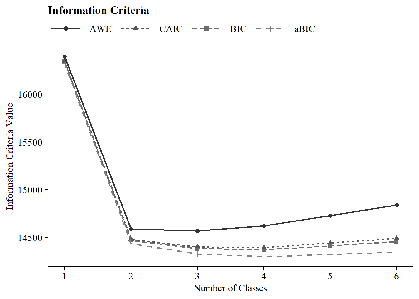
Save figure:
ggsave(here("figures", "info_criteria_moderation.png"), dpi = "retina", bg = "white", height=5, width=7, units="in")7.4.3 Compare Class Solutions
Compare probability plots for \(K = 1:5\) class solutions
model_results <- data.frame()

for (i in 1:length(output_enum)) {
  temp <- output_enum[[i]]$parameters$probability.scale %>%
    mutate(model = paste0(i, "-Class Model"))

  model_results <- rbind(model_results, temp)
}

compare_plot <-
  model_results %>%
  filter(category == 2) %>%
  dplyr::select(est, model, LatentClass, param) %>%
  filter(model != "6-Class Model") #Remove from plot

compare_plot$param <- fct_inorder(compare_plot$param)

ggplot(
  compare_plot,
  aes(
    x = param,
    y = est,
    color = LatentClass,
    shape = LatentClass,
    group = LatentClass,
    lty = LatentClass
  )
) +
  geom_point() +
  geom_line() +
  scale_colour_viridis_d() +
  facet_wrap(~ model, ncol = 2) +
  labs(title = "Math Attitude Items", x = " ", y = "Probability") +
  theme_minimal() +
  theme(panel.grid.major.y = element_blank(),
axis.text.x = element_text(angle = -45, hjust = -.1)) 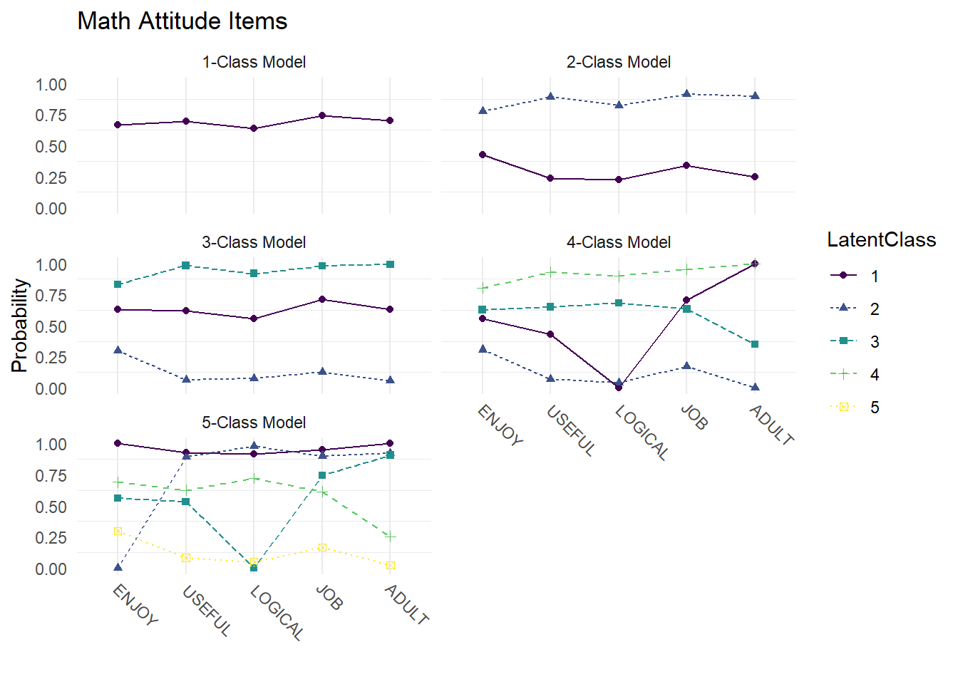
Save figure:
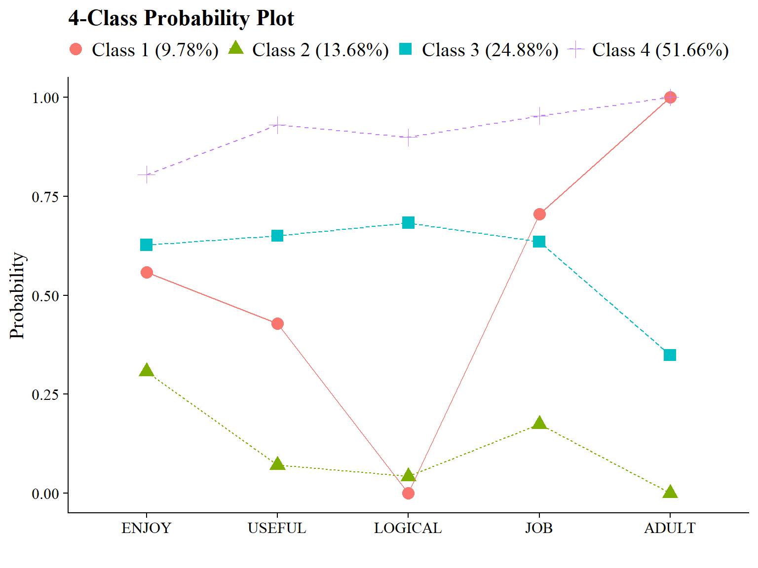
ggsave(here("figures", "compare_kclass_plot_mod.png"), dpi = "retina", bg = "white", height=5, width=7, units="in")7.4.4 4-Class Probability Plot
Use the plot_lca function provided in the folder to plot the item probability plot. This function requires one argument:
- model_name: The name of the Mplus readModels object (e.g., output_lsal$c4_lsal.out)
Save figure:
ggsave(here("figures", "probability_plot_mod.png"), dpi = "retina", bg = "white", height=5, width=7, units="in")7.5 LCA Moderation - ML Three-Step
7.5.1 Step 1 - Estimate Unconditional Model w/ Auxiliary Specification
step1  <- mplusObject(
  TITLE = "Step 1 - Unconditional Model w/ Auxiliary Specification",
  VARIABLE = "categorical = enjoy, useful, logical, job, adult;
  usevar =  enjoy, useful, logical, job, adult;
  classes = c(4);
  AUXILIARY = female math_irt;",

  ANALYSIS =
   "estimator = mlr;
    type = mixture;
    starts = 0;
    OPTSEED = 813779;",

  SAVEDATA =
   "File=savedata.dat;
    Save=cprob;
    format=free;",

  OUTPUT = "sampstat residual tech11 tech14",

  usevariables = colnames(data),
  rdata = data)

step1_fit <- mplusModeler(step1,
                            dataout=here("moderation", "three_step", "new.dat"),
                            modelout=here("moderation", "three_step", "one.inp") ,
check=TRUE, run = TRUE, hashfilename = FALSE)Note: Ensure that the classes did not shift during this step (i.g., Class 1 in the enumeration run is now Class 4). Evaluate output and compare the class counts and proportions for the latent classes. Using the OPTSEED function ensures replication of the best loglikelihood value run.
After selecting the latent class model, add class labels to item probability plot using the plot_lca_labels function. This function requires three arguments:
-
model_name: The MplusreadModelsobject (e.g.,output_lsal$c4_lsal.out) -
item_labels: The item labels for x-axis (e.g.,c(“Enjoy”,“Useful”,“Logical”,“Job”,“Adult”)) -
class_labels: The class labels (e.g., c(“Pro-Science w/ Elevated Utility Value”, “Ambivalent w/ Minimal Utility Value”, “Ambivalent w/ Elevated Utility Value”, “Anti-Science w/ Minimal Utility Value”))
Note: Use \n to add a return if the label is lengthy.
source(here("functions","plot_lca_labels.R"))

# Read in output from step 1.
output_one <- readModels(here("moderation","three_step","one.out"))

# Plot Title
title <- "LCA Probability Plot - LSAL"

#Identify item and class labels (Make sure they are in the order presented in the plot above)
item_labels <-  c(
  "I Enjoy \nScience",
  "Science is Useful \nin Everyday Problems",
  "Science Helps \nLogical Thinking",
  "Need Science for \na Good Job",
  "Will Use Science \nOften as an Adult"
)

class_labels <- c(

  "Ambivalent w/ \nElevated Utility Value",
  "Anti-Science w/ \nMinimal Utility Value",
  "Ambivalent w/ \nMinimal Utility Value",
  "Pro-Science w/ \nElevated Utility Value"
)

# Plot LCA plot
plot_lca_labels(model_name = output_one, item_labels, class_labels, title)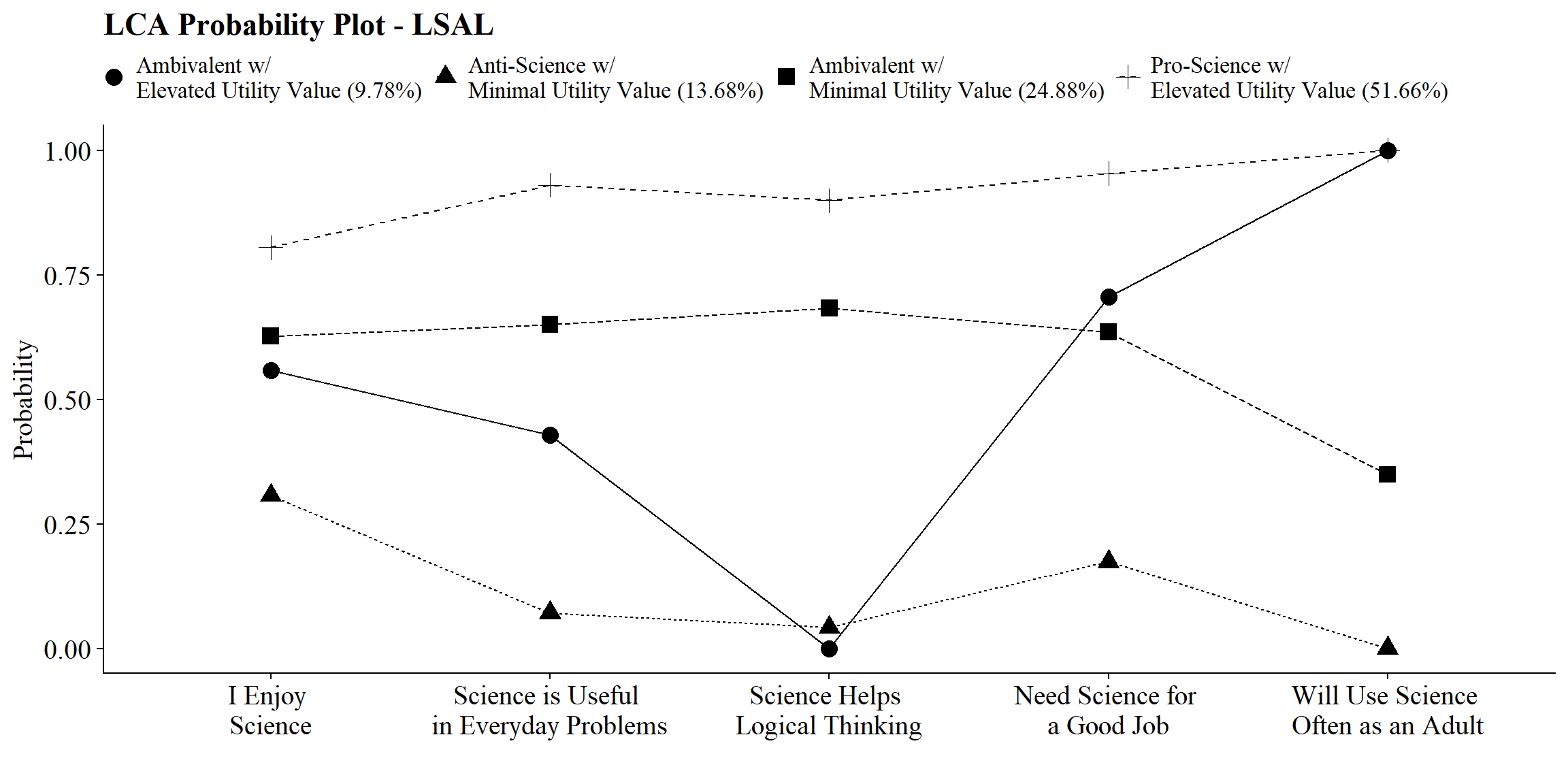
# Save
ggsave(here("figures", "final_probability_plot_mod.png"), dpi = "retina", bg = "white", height=7, width=10, units="in")
7.5.2 Step 2 - Determine Measurement Error
Extract logits for the classification probabilities for the most likely latent class:
logit_cprobs <- as.data.frame(output_one[["class_counts"]]
                                       [["logitProbs.mostLikely"]])
Extract saved dataset from step one:
savedata <- as.data.frame(output_one[["savedata"]])Rename the column in savedata named “C” and change to “N”:
7.5.3 Step 3 - Add Auxiliary Variables
Build the moderation model:
step3mod  <- mplusObject(
  TITLE = "LCA Moderation",

  VARIABLE =
 "nominal=N;
  usevar = n;

  classes = c(4);

  usevar = female math_irt;" ,

  ANALYSIS =
 "estimator = mlr;
  type = mixture;
  starts = 0;",

  MODEL =
  glue(
 "!DISTAL = math_irt, COVARIATE = female, MODERATOR = C

  %OVERALL%
  math_irt on female;
  math_irt;

     %C#1%
  [n#1@{logit_cprobs[1,1]}];
  [n#2@{logit_cprobs[1,2]}];
  [n#3@{logit_cprobs[1,3]}];

  math_irt on female(s1);  ! conditional slope (class 1)
  [math_irt](m1);          ! conditional distal mean
  math_irt;                ! conditional distal variance (freely estimated)

  %C#2%
  [n#1@{logit_cprobs[2,1]}];
  [n#2@{logit_cprobs[2,2]}];
  [n#3@{logit_cprobs[2,3]}];

  math_irt on female(s2);
  [math_irt](m2);
  math_irt;

  %C#3%
  [n#1@{logit_cprobs[3,1]}];
  [n#2@{logit_cprobs[3,2]}];
  [n#3@{logit_cprobs[3,3]}];

  math_irt on female(s3);
  [math_irt](m3);
  math_irt;

  %C#4%
  [n#1@{logit_cprobs[4,1]}];
  [n#2@{logit_cprobs[4,2]}];
  [n#3@{logit_cprobs[4,3]}];

  math_irt on female(s4);
  [math_irt](m4);
  math_irt; "),

  MODELCONSTRAINT =
   "New (
   diff12 diff13 diff23
   diff14 diff24 diff34
   slope12 slope13 slope23
    slope14 slope24 slope34);

    diff12 = m1-m2;  ! test distal outcome differences
    diff13 = m1-m3;
    diff23 = m2-m3;
    diff14 = m1-m4;
    diff24 = m2-m4;
    diff34 = m3-m4;

    slope12 = s1-s2;  ! test pairwise slope differences
    slope13 = s1-s3;
    slope23 = s2-s3;
    slope14 = s1-s4;
    slope24 = s2-s4;
    slope34 = s3-s4;",

  MODELTEST = " ! can run only a single Omnibus test per model
    s1=s2;
    s2=s3;
    s3=s4;",

  usevariables = colnames(savedata),
  rdata = savedata)

step3mod_fit <- mplusModeler(step3mod,
               dataout=here("moderation", "three_step", "mod.dat"),
               modelout=here("moderation", "three_step", "three.inp"),
check=TRUE, run = TRUE, hashfilename = FALSE)| Latent Class | Label |
|---|---|
| 1 | Ambivalent with Elevated Utility Value |
| 2 | Anti-Science with Minimal Utility Value |
| 3 | Ambivalent with Minimal Utility Value |
| 4 | Pro-Science with Elevated Utility Value |
7.5.3.1 Wald Test Table
modelParams <- readModels(here("moderation", "three_step", "three.out"))

# Extract information as data frame
wald <- as.data.frame(modelParams[["summaries"]]) %>%
  dplyr::select(WaldChiSq_Value:WaldChiSq_PValue) %>%
  mutate(WaldChiSq_DF = paste0("(", WaldChiSq_DF, ")")) %>%
  unite(wald_test, WaldChiSq_Value, WaldChiSq_DF, sep = " ") %>%
  rename(pval = WaldChiSq_PValue) %>%
  mutate(pval = ifelse(pval<0.001, paste0(".001*"),
                       ifelse(pval<0.05, paste0(scales::number(pval, accuracy = .001), "*"),
                              scales::number(pval, accuracy = .001))))

# Create table

wald %>%
  gt() %>%
    tab_header(
    title = "Wald Test of Paramter Constraints (Slope)") %>%
    cols_label(
      wald_test = md("Wald Test (*df*)"),
      pval = md("*p*-value")) %>%
  cols_align(align = "center") %>%
  opt_align_table_header(align = "left") %>%
gt::tab_options(table.font.names = "serif")| Wald Test of Paramter Constraints (Slope) | |
| Wald Test (df) | p-value |
|---|---|
| 12.613 (3) | 0.006* |
7.5.3.2 Table of Slope and Intercept Values Across Classes
modelParams <- readModels(here("moderation", "three_step", "three.out"))

# Change these to how the variables are written in Mplus
x <- "FEMALE"
y <- "MATH_IRT"

# Extract information as data frame
values <- as.data.frame(modelParams[["parameters"]][["unstandardized"]]) %>%
  filter(param %in% c(x, y),
         paramHeader != "Residual.Variances") %>%
  mutate(param = str_replace(param, pattern = x, replacement = "Slope"),
         param = str_replace(param, pattern = y, replacement = "Intercept")) %>%
  mutate(LatentClass = sub("^","Class ", LatentClass)) %>%
  dplyr::select(!paramHeader) %>%
  mutate(se = paste0("(", format(round(se,2), nsmall =2), ")")) %>%
    unite(estimate, est, se, sep = " ") %>%
  select(!est_se) %>%
  mutate(pval = ifelse(pval<0.001, paste0("<.001*"),
                       ifelse(pval<0.05, paste0(scales::number(pval, accuracy = .001), "*"),
                              scales::number(pval, accuracy = .001))))


# Create table

values %>%
  gt(groupname_col = "LatentClass", rowname_col = "param") %>%
  tab_header(
    title = "Slope and Intercept Values Across Science Attitudes Classes") %>%
  cols_label(
    estimate = md("Estimate (*se*)"),
    pval = md("*p*-value")) %>%
  sub_values(values = "999.000", replacement = "-") %>%
  sub_missing(1:3,
              missing_text = "") %>%
  cols_align(align = "center") %>%
  opt_align_table_header(align = "left") %>%
gt::tab_options(table.font.names = "serif")| Slope and Intercept Values Across Science Attitudes Classes | ||
| Estimate (se) | p-value | |
|---|---|---|
| Class 1 | ||
| Slope | -4.452 (2.60) | 0.086 |
| Intercept | 55.966 (1.29) | <.001* |
| Class 2 | ||
| Slope | -4.475 (1.85) | 0.015* |
| Intercept | 56.729 (1.12) | <.001* |
| Class 3 | ||
| Slope | -2.678 (1.76) | 0.128 |
| Intercept | 59.265 (0.80) | <.001* |
| Class 4 | ||
| Slope | 1.097 (0.87) | 0.206 |
| Intercept | 60.725 (0.51) | <.001* |
7.5.3.3 Table of Distal Outcome Differences
modelParams <- readModels(here("moderation", "three_step", "three.out"))

# Extract information as data frame
diff <- as.data.frame(modelParams[["parameters"]][["unstandardized"]]) %>%
  filter(grepl("DIFF", param)) %>%
  dplyr::select(param:pval) %>%
  mutate(se = paste0("(", format(round(se,2), nsmall =2), ")")) %>%
  unite(estimate, est, se, sep = " ") %>%
  mutate(param = str_remove(param, "DIFF"),
         param = as.numeric(param)) %>%
  separate(param, into = paste0("Group", 1:2), sep = 1) %>%
  mutate(class = paste0("Class ", Group1, " vs ", Group2)) %>%
  select(class, estimate, pval)


# Create table

diff %>%
  gt() %>%
    tab_header(
    title = "Distal Outcome Differences") %>%
    cols_label(
      class = "Class",
      estimate = md("Mean (*se*)"),
      pval = md("*p*-value")) %>%
    sub_missing(1:3,
              missing_text = "") %>%
  fmt(3,
    fns = function(x)
      ifelse(x<0.05, paste0(scales::number(x, accuracy = .001), "*"),
             scales::number(x, accuracy = .001))
  ) %>%
  cols_align(align = "center") %>%
  opt_align_table_header(align = "left") %>%
gt::tab_options(table.font.names = "serif")| Distal Outcome Differences | ||
| Class | Mean (se) | p-value |
|---|---|---|
| Class 1 vs 2 | -0.763 (1.70) | 0.654 |
| Class 1 vs 3 | -3.299 (1.57) | 0.035* |
| Class 2 vs 3 | -2.536 (1.45) | 0.081 |
| Class 1 vs 4 | -4.759 (1.43) | 0.001* |
| Class 2 vs 4 | -3.996 (1.23) | 0.001* |
| Class 3 vs 4 | -1.46 (1.00) | 0.143 |
7.5.3.4 Table of Slope Differences
modelParams <- readModels(here("moderation", "three_step", "three.out"))

# Extract information as data frame
diff2 <- as.data.frame(modelParams[["parameters"]][["unstandardized"]]) %>%
  filter(grepl("SLOPE", param)) %>%
  dplyr::select(param:pval) %>%
  mutate(se = paste0("(", format(round(se,2), nsmall =2), ")")) %>%
  unite(estimate, est, se, sep = " ") %>%
  mutate(param = str_remove(param, "SLOPE"),
         param = as.numeric(param)) %>%
  separate(param, into = paste0("Group", 1:2), sep = 1) %>%
  mutate(class = paste0("Class ", Group1, " vs ", Group2)) %>%
  select(class, estimate, pval) %>%
  mutate(pval = ifelse(pval<0.001, paste0("<.001*"),
                       ifelse(pval<0.05, paste0(scales::number(pval, accuracy = .001), "*"),
                              scales::number(pval, accuracy = .001))))


# Create table

diff2 %>%
  gt() %>%
    tab_header(
    title = "Slope Differences") %>%
    cols_label(
      class = "Class",
      estimate = md("Mean (*se*)"),
      pval = md("*p*-value")) %>%
    sub_missing(1:3,
              missing_text = "") %>%
  cols_align(align = "center") %>%
  opt_align_table_header(align = "left") %>%
gt::tab_options(table.font.names = "serif")| Slope Differences | ||
| Class | Mean (se) | p-value |
|---|---|---|
| Class 1 vs 2 | 0.023 (3.08) | 0.994 |
| Class 1 vs 3 | -1.774 (3.46) | 0.608 |
| Class 2 vs 3 | -1.797 (2.92) | 0.538 |
| Class 1 vs 4 | -5.549 (2.83) | 0.050 |
| Class 2 vs 4 | -5.572 (1.97) | 0.005* |
| Class 3 vs 4 | -3.775 (2.16) | 0.080 |
7.5.3.5 Table of Covariates
modelParams <- readModels(here("moderation", "three_step", "three.out"))

x <- "FEMALE"
rename <- "Gender"

# Extract information as data frame
cov <- as.data.frame(modelParams[["parameters"]][["unstandardized"]]) %>%
  filter(param %in% c(x)) %>%
  mutate(param = str_replace(param, x, rename)) %>%
  mutate(LatentClass = sub("^","Class ", LatentClass)) %>%
  dplyr::select(!paramHeader) %>%
  mutate(se = paste0("(", format(round(se,2), nsmall =2), ")")) %>%
    unite(estimate, est, se, sep = " ") %>%
  select(param, estimate, pval) %>%
  distinct(param, .keep_all=TRUE)  %>%
  mutate(pval = ifelse(pval<0.001, paste0("<.001*"),
                       ifelse(pval<0.05, paste0(scales::number(pval, accuracy = .001), "*"),
                              scales::number(pval, accuracy = .001))))


# Create table

cov %>%
  gt(groupname_col = "LatentClass", rowname_col = "param") %>%
  tab_header(
    title = "Relations Between the Covariates and Distal Outcome") %>%
  cols_label(
    estimate = md("Estimate (*se*)"),
    pval = md("*p*-value")) %>%
  sub_missing(1:3,
              missing_text = "") %>%
  sub_values(values = c(999.000), replacement = "-") %>%
  cols_align(align = "center") %>%
  opt_align_table_header(align = "left") %>%
gt::tab_options(table.font.names = "serif")| Relations Between the Covariates and Distal Outcome | ||
| Estimate (se) | p-value | |
|---|---|---|
| Gender | -4.452 (2.60) | 0.086 |
7.5.3.6 Plot Distal Outcome
modelParams <- readModels(here("moderation", "three_step", "three.out"))

y <- "MATH_IRT"

# Extract class size
c_size <- as.data.frame(modelParams[["class_counts"]][["modelEstimated"]][["proportion"]]) %>%
  rename("cs" = 1) %>%
  mutate(cs = round(cs*100, 2))

# Keep this code if you want a generic label for the classes
#c_size_val <- paste0("C", 1:nrow(c_size), glue(" ({c_size[1:nrow(c_size),]}%)"))

# Otherwise use this:
c_size_val <- paste0(class_labels, glue(" ({c_size[1:nrow(c_size),]}%)"))


# Extract information as data frame
estimates <- as.data.frame(modelParams[["parameters"]][["unstandardized"]]) %>%
  filter(paramHeader == "Intercepts") %>%
  dplyr::select(param, est, se) %>%
  filter(param == y) %>%
  mutate(across(c(est, se), as.numeric)) %>%
  mutate(LatentClass = c_size_val)

# Plot bar graphs
estimates %>%
  ggplot(aes(x=LatentClass, y = est, fill = LatentClass)) +
  geom_col(position = "dodge", stat = "identity", color = "black") +
  geom_errorbar(aes(ymin=est-se, ymax=est+se),
                size=.3,    # Thinner lines
                width=.2,
                position=position_dodge(.9)) +
  geom_text(aes(label = est),
            family = "serif", size = 4,
            position=position_dodge(.9),
            vjust = 8) +
  #scale_fill_grey(start = .4, end = .7) +
  labs(y="Math Score", x="") +
  theme_cowplot() +
  theme(text = element_text(family = "serif", size = 12),
        axis.text.x = element_text(size=12),
        legend.position="none") +
  coord_cartesian(ylim=c(0,80),  # Change ylim based on distal outcome range
expand = FALSE) 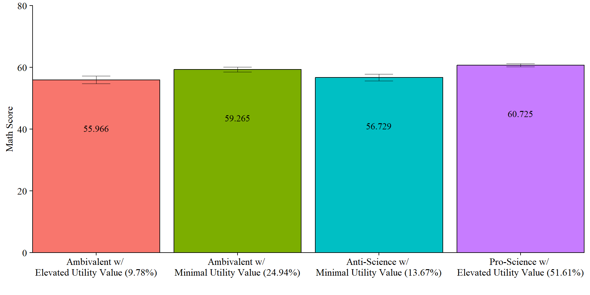
# Save plot
ggsave(here("figures","distal_plot_mod.jpeg"), dpi = "retina", bg = "white", width=10, height = 7, units="in")
7.5.4 Plot Interaction
7.5.4.1 Bar plot
modelParams <- readModels(here("moderation", "three_step", "three.out"))

x <- "FEMALE"

# Extract information as data frame
desc <- as.data.frame(modelParams$sampstat$univariate.sample.statistics) %>%
  rownames_to_column("Variables")

# Select min amd max values of covariate
xmin <- desc %>%
  filter(Variables == x) %>%
  dplyr::select(Minimum) %>%
  as.numeric()
xmax <- desc %>%
  filter(Variables == x) %>%
  dplyr::select(Maximum) %>%
  as.numeric()

# Add slope and intercept, Min and Max values
line <- as.data.frame(modelParams$parameters$unstandardized) %>%
  filter(str_detect(paramHeader, 'ON|Inter')) %>%
  unite("param", paramHeader:param, remove = TRUE) %>%
  mutate(param = replace(param,agrep(".ON",param),"slope"),
         param = replace(param,agrep("Inter", param), "intercept"),
         LatentClass = factor(LatentClass, labels = c_size_val)) %>%
  dplyr::select(param, est, LatentClass) %>%
  pivot_wider(names_from = param, values_from = est) %>%
  add_column(x_max = xmax,
         x_min = xmin)


# Add column with y values
data <- line %>%
  mutate(y_min = (slope*xmin) + intercept,
         y_max = (slope*xmax) + intercept) %>%
  dplyr::select(-slope, -intercept) %>%
  pivot_longer(-LatentClass,
               names_to = c("xvalues", "yvalues"),
               names_sep="_" ) %>%
  pivot_wider(names_from = xvalues, values_from = value) %>%
  dplyr::select(-yvalues) %>%
  mutate(x = case_when(
           x == 1 ~ "Female", ## Change these names
           x == 0 ~ "Male")) ## Change these names

# Plot bar graphs
data %>%
  ggplot(aes(x=factor(x), y = y, fill = LatentClass)) +
  geom_col(position = "dodge", stat = "identity", color = "black") +
  geom_text(aes(label = y),
            family = "serif", size = 4,
            position=position_dodge(.9),
            vjust = -.5) +
  #scale_fill_grey(start = .4, end = .7) +
  labs(y="Math Score", x="") +
  theme_cowplot() +
  theme(text = element_text(family = "serif", size = 12),
        axis.text.x = element_text(size=12)) +
  coord_cartesian(ylim=c(0,80),  # Change ylim based on distal outcome range
expand = FALSE) 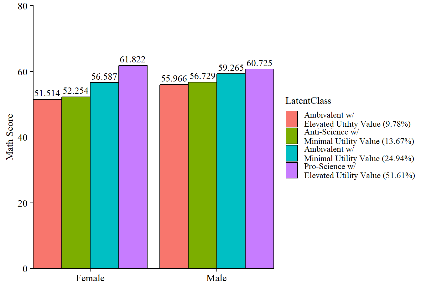
# Save plot
ggsave(here("figures","interaction_mod.jpeg"), dpi = "retina", bg = "white", width=10, height = 7, units="in")
7.5.4.2 Line plot
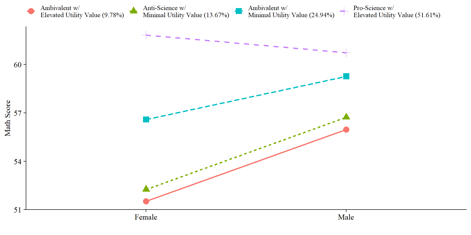
Here we can visualize the slopes.
x <- "FEMALE"

# Minimum and Maximum Values
desc <- as.data.frame(modelParams$sampstat$univariate.sample.statistics) %>%
  rownames_to_column("Variables")


# Select min amd max values of covariate
xmin <- desc %>%
  filter(Variables == x) %>%
  dplyr::select(Minimum) %>%
  as.numeric()
xmax <- desc %>%
  filter(Variables == x) %>%
  dplyr::select(Maximum) %>%
  as.numeric()

# Add slope and intercept, Min and Max values
line <- as.data.frame(modelParams$parameters$unstandardized) %>%
  filter(str_detect(paramHeader, 'ON|Inter')) %>%
  unite("param", paramHeader:param, remove = TRUE) %>%
  mutate(param = replace(param,agrep(".ON",param),"slope"),
         param = replace(param,agrep("Inter", param), "intercept"),
         LatentClass = factor(LatentClass, labels = c_size_val)) %>%
  dplyr::select(param, est, LatentClass) %>%
  pivot_wider(names_from = param, values_from = est) %>%
  add_column(x_max = xmax,
         x_min = xmin)


# Add column with y values
data <- line %>%
  mutate(y_min = (slope*xmin) + intercept,
         y_max = (slope*xmax) + intercept) %>%
  dplyr::select(-slope, -intercept) %>%
  pivot_longer(-LatentClass,
               names_to = c("xvalues", "yvalues"),
               names_sep="_" ) %>%
  pivot_wider(names_from = xvalues, values_from = value) %>%
  dplyr::select(-yvalues) %>%
  mutate(x = case_when(
           x == 1 ~ "Female",
           x == 0 ~ "Male"))

# Plot
data %>%
  ggplot(aes(
    x = factor(x),
    y = y,
    color = LatentClass,
    group = LatentClass,
    lty = LatentClass,
    shape = LatentClass
  )) +
  geom_point(size = 4) +
  geom_line(aes(group = LatentClass), size = 1) +
  labs(x = "",
       y = "Math Score") +
  #scale_colour_grey(start = .3, end = .6) +
  theme_cowplot() +
  theme(
    text = element_text(family = "serif", size = 12),
    axis.text.x = element_text(size = 12),
    legend.text = element_text(family = "serif", size = 10),
    legend.position = "top",
    legend.title = element_blank()
) 
# Save
ggsave(here("figures","slope_plot_mod.jpeg"),  dpi = "retina", bg = "white", width=10, height = 7, units="in")
It’s also important to report the slope coefficients. Which ones would you assume are significant based on the plots?