29 Comparing Cluster Analysis and Latent Profile Analysis (B. J. Yik,* Y. Zhang, K. Nylund-Gibson, M. Ing, L. Krawiec, J. D. Houck, & E. D. Nacsa, 2026)

Citation: Exploring Heterogeneity in Chemistry Education Research: Comparing Cluster Analysis and Latent Profile Analysis (B. J. Yik,* Y. Zhang, K. Nylund-Gibson, M. Ing, L. Krawiec, J. D. Houck, & E. D. Nacsa (2026)

library(tidyverse)
library(haven)
library(glue)
library(MplusAutomation)
library(rhdf5)
library(here)
library(janitor)
library(semPlot)
library(reshape2)
library(cowplot)
library(filesstrings)
library(hrbrthemes)
library(sjPlot)
library(dplyr)
library(naniar)
library(gt)
library(tidyLPA)
#library(pisaUSA15)
library(patchwork)
library(RcppAlgos)
library(DiagrammeR)
library(data.table)
library(poLCA)
library(cluster)
library(factoextra)
library(datasets)
library(Hmisc)
library(car)

Proposed model applied in current study

grViz(" digraph lca_model {

# The `graph` statement - No editing needed

    graph [layout = dot, overlap = true]
 
# Two `node` statements
 
# One for measured variables (box) 

    node [shape=box]
    Attitudes [label = <Attitudes toward <br/>chemistry>]
    Motivation
    Effort [label = <Effort Beliefs>]
    Efficacy [label = <Self-efficacy>] 
    Concept [label = <Self-concept>]
    Grading [label = <Grading Scheme>]
    Exam [label = <ACS Exam Score>];
 
# One for latent variables (circle) 
 
    node [shape=circle]
    dispositions [label=<Student <br/>Affects <br/>C<sub>k=3</sub>>];
    
# `edge` statements
 
    edge [minlen = 2]
    dispositions -> {Attitudes Motivation Effort Efficacy Concept}
    dispositions -> Exam [minlen = 4];
    Grading -> dispositions [minlen = 4];
    Grading -> Exam;
    
 {rank = same; Grading; dispositions; Exam}
 #{rank = source; Attitudes; Motivation; Effort; Efficacy; Concept}
 }")

load the dataset

#load data
pre <- read.csv(here("33-k-means", "grading-pre-v2.csv"))

handling missing data

#any(is.na(pre))
pre_clean <- pre %>% drop_na()
any(is.na(pre_clean))
#> [1] FALSE

#we also cleaned out this few datapoint, since we previously included race as an auxiliary variable, but deleted after; but we did not change the sample for LPA. only 6 sample was deleted due to this step 
pre_clean <- pre_clean %>%
  filter(!Gender %in% c("I am gender nonconforming,I am genderqueer or genderfluid", "My gender or gender identity is best described as:", "I am gender nonconforming", "I prefer not to disclose my gender or gender identity", "I am genderqueer or genderfluid", "I am nonbinary" ))

view data

recode

pre_clean <- pre_clean %>%
  mutate(grading = ifelse(grading == "specs", 1, 0))  # specs = 1, trad = 0

calculate means for each scale

pre_clean <- pre_clean %>%
  mutate(ASCI_IA = rowMeans(across(c(ASCI1:ASCI8)), na.rm = TRUE)) %>%
  mutate(AMSC = rowMeans(across(c(AMSC01:AMSC28)), na.rm = TRUE)) %>%
  mutate(EB = rowMeans(across(c(EBN1:EBP4)), na.rm = TRUE)) %>%
  mutate(MSLQ = rowMeans(across(c(MSLQ05:MSLQ31)), na.rm = TRUE)) %>%
  mutate(CSC = rowMeans(across(c(CSC24:CSC08)), na.rm = TRUE))

#update the data preview
sjPlot::view_df(pre_clean)

Data frame: pre_clean
ID	Name	Values	Value Labels
1	ID		<output omitted>
2	grading	range: 0-1
3	exam	range: 34-100
4	mark		<output omitted>
5	ASCI1	range: 2-7
6	ASCI2	range: 1-7
7	ASCI3	range: 1-7
8	ASCI4	range: 1-7
9	ASCI5	range: 1-7
10	ASCI6	range: 1-7
11	ASCI7	range: 1-7
12	ASCI8	range: 1-7
13	AMSC01	range: 1-5
14	AMSC02	range: 1-5
15	AMSC03	range: 1-5
16	AMSC04	range: 1-5
17	AMSC05	range: 1-5
18	AMSC06	range: 1-5
19	AMSC07	range: 1-5
20	AMSC08	range: 1-5
21	AMSC09	range: 1-5
22	AMSC10	range: 1-5
23	AMSC11	range: 1-5
24	AMSC12	range: 1-5
25	AMSC13	range: 1-5
26	AMSC14	range: 1-5
27	AMSC15	range: 1-5
28	AMSC16	range: 1-5
29	AMSC17	range: 1-5
30	AMSC18	range: 1-5
31	AMSC19	range: 1-5
32	AMSC20	range: 1-5
33	AMSC21	range: 1-5
34	AMSC22	range: 1-5
35	AMSC23	range: 1-5
36	AMSC24	range: 1-5
37	AMSC25	range: 1-5
38	AMSC26	range: 1-5
39	AMSC27	range: 1-5
40	AMSC28	range: 1-5
41	EBN1	range: 1-5
42	EBN2	range: 1-5
43	EBN3	range: 1-5
44	EBN4	range: 1-5
45	EBN5	range: 1-5
46	EBP1	range: 1-5
47	EBP2	range: 1-5
48	EBP3	range: 1-5
49	EBP4	range: 1-5
50	MSLQ05	range: 1-5
51	MSLQ06	range: 1-5
52	MSLQ12	range: 1-5
53	MSLQ15	range: 1-5
54	MSLQ20	range: 1-5
55	MSLQ21	range: 1-5
56	MSLQ29	range: 1-5
57	MSLQ31	range: 1-5
58	CSC24	range: 1-5
59	CSC28	range: 1-5
60	CSC20	range: 1-5
61	CSC36	range: 1-5
62	CSC16	range: 1-5
63	CSC40	range: 1-5
64	CSC04	range: 1-5
65	CSC12	range: 1-5
66	CSC32	range: 1-5
67	CSC08	range: 1-5
68	Age	range: 18-25
69	Major		<output omitted>
70	Year		<output omitted>
71	Year_6_TEXT
72	Credits.		<output omitted>
73	Work		<output omitted>
74	FirstGen		<output omitted>
75	Gender		<output omitted>
76	Gender.1		<output omitted>
77	Race		<output omitted>
78	Race._8_TEXT
79	ASCI_IA	range: 2.1-5.8
80	AMSC	range: 1.6-4.3
81	EB	range: 1.0-4.3
82	MSLQ	range: 1.0-5.0
83	CSC	range: 1.8-4.8

standardize the variables (z-score)

pre_clean <- pre_clean %>%
  mutate(across(all_of(c("ASCI_IA", "AMSC", "EB", "MSLQ", "CSC")), ~ scale(.)[,1], .names = "z_{.col}"))

double check all indicators are standardized

ds <- pre_clean %>%
    pivot_longer(z_ASCI_IA:z_CSC, names_to = "variable") %>%
    group_by(variable) %>%
    summarise(mean = mean(value, na.rm = TRUE), sd = sd(value, na.rm = TRUE))

ds %>%
    gt() %>%
    tab_header(title = md("**Descriptive Summary**")) %>%
    cols_label(variable = "Variable", mean = md("M"), sd = md("SD")) %>%
    fmt_number(c(2:3), decimals = 2) %>%
    cols_align(align = "center", columns = mean)

Variable	M	SD
Descriptive Summary
z_AMSC	0.00	1.00
z_ASCI_IA	0.00	1.00
z_CSC	0.00	1.00
z_EB	0.00	1.00
z_MSLQ	0.00	1.00


data_long <- pre_clean %>%
    pivot_longer(z_ASCI_IA:z_CSC, names_to = "variable")

ggplot(data_long, aes(x = value)) + geom_histogram(binwidth = 0.3, fill = "#69b3a2",
    color = "black") + facet_wrap(~variable, scales = "free_x") + labs(title = "Histograms of Variables",
    x = "Value", y = "Frequency") + theme_cowplot()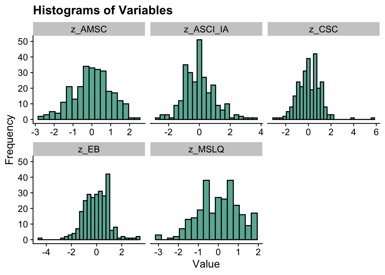

correlations

df_cor <- pre_clean %>%
  dplyr::select(z_ASCI_IA, z_AMSC, z_EB, z_MSLQ, z_CSC, grading, exam)

cor_matrix <- cor(df_cor, use = "pairwise.complete.obs")

print(cor_matrix)
#>             z_ASCI_IA      z_AMSC        z_EB     z_MSLQ
#> z_ASCI_IA  1.00000000 -0.27197825  0.14356191 -0.1530685
#> z_AMSC    -0.27197825  1.00000000  0.01863942  0.2160171
#> z_EB       0.14356191  0.01863942  1.00000000 -0.3713385
#> z_MSLQ    -0.15306849  0.21601714 -0.37133853  1.0000000
#> z_CSC      0.10072946  0.16121343  0.33859758 -0.1155573
#> grading    0.05509749 -0.08774336  0.07088039  0.1083377
#> exam      -0.15544345  0.02709785 -0.21220105  0.3720302
#>                 z_CSC     grading        exam
#> z_ASCI_IA  0.10072946  0.05509749 -0.15544345
#> z_AMSC     0.16121343 -0.08774336  0.02709785
#> z_EB       0.33859758  0.07088039 -0.21220105
#> z_MSLQ    -0.11555730  0.10833767  0.37203022
#> z_CSC      1.00000000  0.11970707 -0.02177322
#> grading    0.11970707  1.00000000  0.11708381
#> exam      -0.02177322  0.11708381  1.00000000

cor_result <- rcorr(as.matrix(df_cor))

formatted_p <- formatC(cor_result$P, format = "f", digits = 2)

dim(formatted_p) <- dim(cor_result$P)
rownames(formatted_p) <- colnames(formatted_p) <- colnames(df_cor)

print(formatted_p, quote = FALSE)
#>           z_ASCI_IA z_AMSC z_EB z_MSLQ z_CSC grading exam
#> z_ASCI_IA  NA       0.00   0.02 0.01   0.10  0.37    0.01
#> z_AMSC    0.00       NA    0.76 0.00   0.01  0.15    0.66
#> z_EB      0.02      0.76    NA  0.00   0.00  0.25    0.00
#> z_MSLQ    0.01      0.00   0.00  NA    0.06  0.08    0.00
#> z_CSC     0.10      0.01   0.00 0.06    NA   0.05    0.72
#> grading   0.37      0.15   0.25 0.08   0.05   NA     0.06
#> exam      0.01      0.66   0.00 0.00   0.72  0.06     NA

run LPA model

# Run LPA models (no need to run it everytime)
lpa_fit <- pre_clean %>%
    dplyr::select(z_ASCI_IA, z_AMSC, z_EB, z_MSLQ, z_CSC) %>%
    estimate_profiles(1:6, package = "MplusAutomation", ANALYSIS = "starts = 500 100;",
        OUTPUT = "sampstat residual tech11 tech14", variances = c("equal", "varying",
            "equal", "varying"), covariances = c("zero", "zero",
            "equal", "varying"), keepfiles = TRUE)

#compare fit statistics
get_fit(lpa_fit)

# Move files to folder
files <- list.files(here(), pattern = "^model")
move_files(files, here("33-k-means", "new"), overwrite = TRUE)

source(here("33-k-means", "functions", "enum_table_lpa.r")) #file in the folder

# Read in model
output_pisa <- readModels(here("33-k-means", "new"), quiet = TRUE)

# Preview with numbered rows
enum_fit(output_pisa)

model fit summary table (this is the old version table, still working on the new one; the new one will include smallest profile)

select_models <-LatexSummaryTable(output_pisa,                                 
                keepCols=c("Title", "Parameters", "LL", "BIC", "aBIC",
                           "BLRT_PValue", "T11_VLMR_PValue","Observations"))

enum_table(select_models, 1:6, 7:12, 13:18, 19:23)

source(here("33-k-means", "functions","ic_plot_lpa.R")) 
#file in the folder
ic_plot(output_pisa)

second round comparison among different profiles

# CmpK recalculation:
enum_fit1 <- select_models

stage2_cmpk <- enum_fit1 %>% 
  slice(2, 3, 6, 8, 12, 16, 20, 22) %>% # Change this to select the rows of the candidate models
  mutate(CAIC = -2 * LL + Parameters * (log(Observations) + 1)) %>%
  mutate(AWE = -2 * LL + 2 * Parameters * (log(Observations) + 1.5)) %>%
  mutate(SIC = -.5 * BIC,
         expSIC = exp(SIC - max(SIC)),
         cmPk = expSIC / sum(expSIC),
         BF = exp(SIC - lead(SIC)))  %>%
  dplyr::select(Title, Parameters, BIC, aBIC, CAIC, AWE, cmPk, BF) %>%
  mutate(Title = str_to_title(Title)) 

# Format Fit Table
stage2_cmpk %>%
  gt() %>% 
  tab_options(column_labels.font.weight = "bold") %>%
  fmt_number(
    7,
    decimals = 2,
    drop_trailing_zeros = TRUE,
    suffixing = TRUE
  ) %>%
  fmt_number(c(3:6),
             decimals = 2) %>% 
    fmt_number(8,decimals = 2,
             drop_trailing_zeros=TRUE,
             suffixing = TRUE) %>% 
  fmt(8, fns = function(x) 
    ifelse(x>100, ">100",
           scales::number(x, accuracy = .1))) %>% 
  tab_style(
    style = list(
      cell_text(weight = "bold")
      ),
    locations = list(cells_body(
     columns = BIC,
     row = BIC == min(BIC[1:nrow(stage2_cmpk)]) 
    ),
    cells_body(
     columns = aBIC,
     row = aBIC == min(aBIC[1:nrow(stage2_cmpk)])
    ),
    cells_body(
     columns = CAIC,
     row = CAIC == min(CAIC[1:nrow(stage2_cmpk)])
    ),
    cells_body(
     columns = AWE,
     row = AWE == min(AWE[1:nrow(stage2_cmpk)])
    ),
    cells_body(
     columns = cmPk,
     row =  cmPk == max(cmPk[1:nrow(stage2_cmpk)])
     ),
    cells_body(
     columns = BF, 
     row =  BF > 10)
  )
)

Title	Parameters	BIC	aBIC	CAIC	AWE	cmPk	BF
Model 1 With 2 Classes	16	3,820.72	3,769.99	3,836.72	3,958.24	NA	0.2
Model 1 With 3 Classes	22	3,817.02	3,747.27	3,839.02	4,006.11	NA	>100
Model 1 With 6 Classes	40	3,842.50	3,715.68	3,882.50	4,186.29	NA	0.0
Model 2 With 2 Classes	21	3,831.49	3,764.91	3,852.49	4,011.98	NA	>100
Model 2 With 6 Classes	65	3,922.35	3,716.26	3,987.35	4,481.01	NA	0.0
Model 3 With 4 Classes	38	3,817.99	3,697.51	3,855.99	4,144.59	NA	0.9
Model 6 With 2 Classes	41	3,817.80	3,687.80	3,858.80	4,170.18	NA	NA
Model 6 With 4 Classes	NA	NA	NA	NA	NA	NA	NA

Comparing two profiles

a <- plotMixtures(output_pisa$model_2_class_2.out, ci = 0.95, bw = FALSE)

b <- plotMixtures(output_pisa$model_6_class_2.out, ci = 0.95, bw = FALSE)

a + labs(title = "Model 2 two-profile") + theme(plot.title = element_text(size = 12)) + b + labs(title = "Model 4 two-profile") +
    theme(plot.title = element_text(size = 12))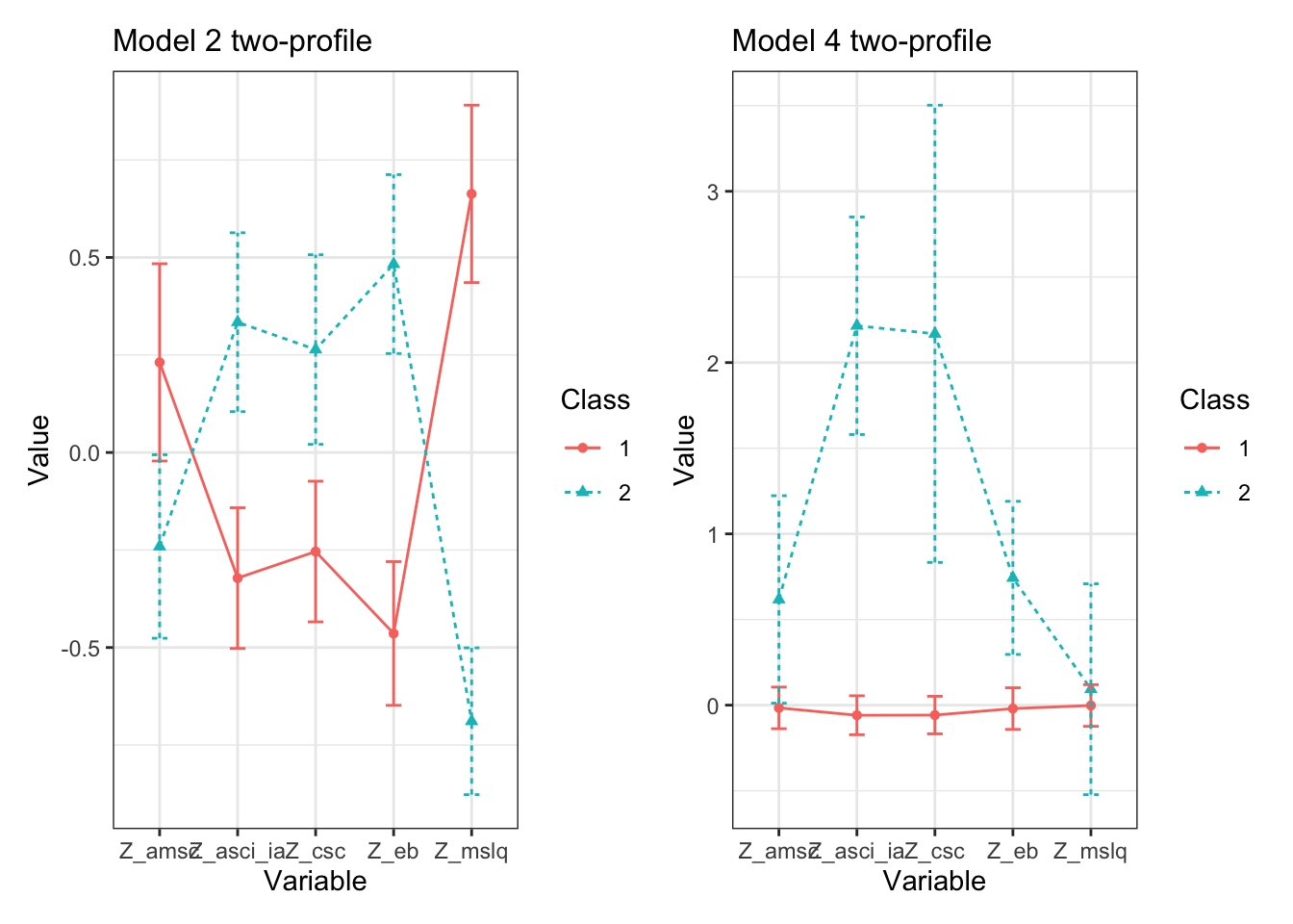

a initial look, not the final figure

source(here("33-k-means", "functions", "plot_lpa.R"))  #file in the folder

plot_lpa(model_name = output_pisa$model_2_class_2.out)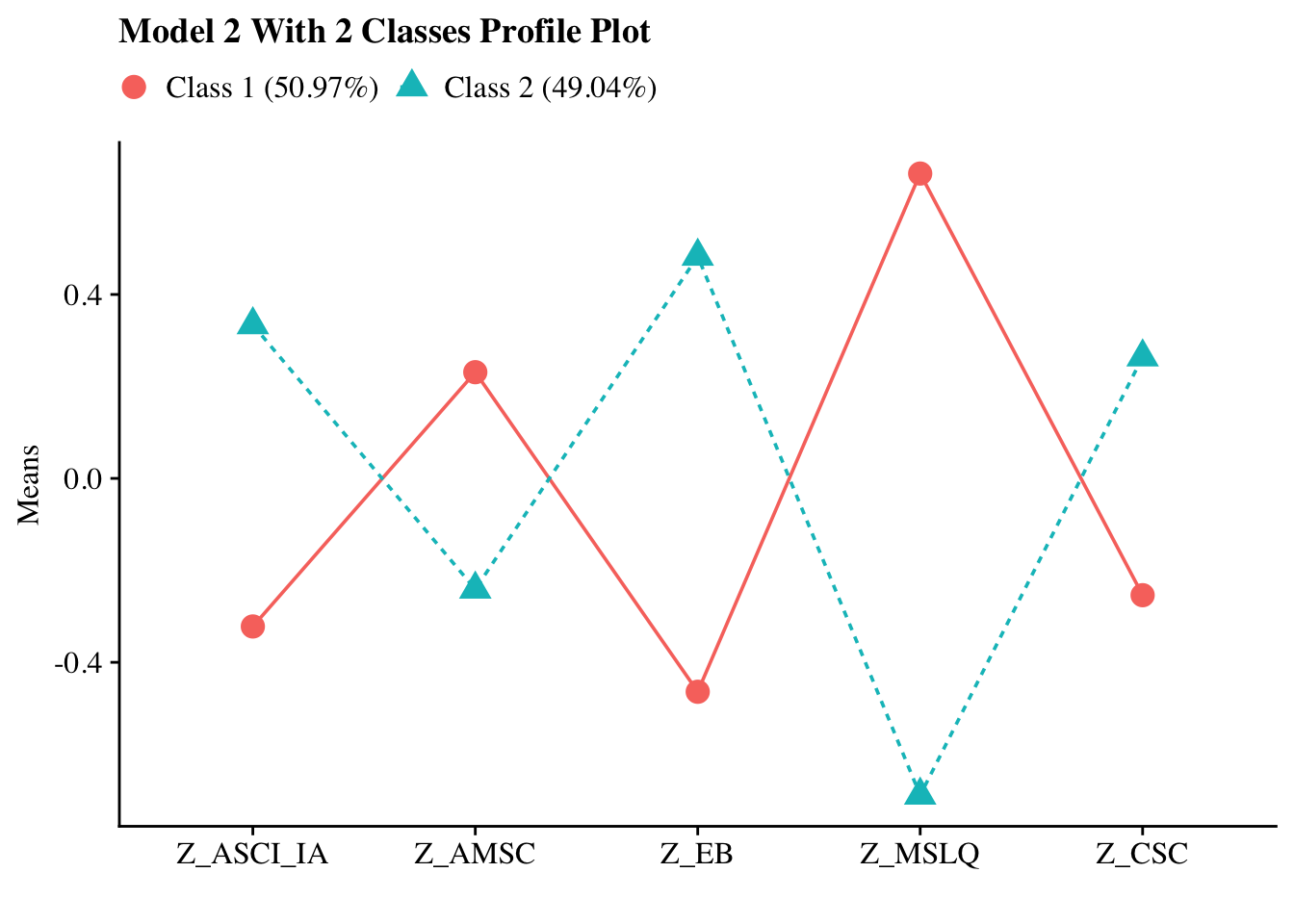

another version: this one changed the color of two profiles and the variable names (all labels)

plot_lpa <- function(model_name) {

  # Extract and reshape mean estimates by class
  pp_plots <- data.frame(model_name$parameters$unstandardized) %>%
    mutate(LatentClass = sub("^", "Class ", LatentClass)) %>%
    filter(paramHeader == "Means") %>%
    filter(LatentClass != "Class Categorical.Latent.Variables") %>%
    dplyr::select(est, LatentClass, param) %>%
    pivot_wider(names_from = LatentClass, values_from = est) %>%
    relocate(param, .after = last_col())
  
  # Extract class proportions
  c_size <- as.data.frame(model_name$class_counts$modelEstimated$proportion) %>%
    dplyr::rename("cs" = 1) %>%
    mutate(cs = round(cs * 100, 2))
  
  # Rename class labels with proportions
# Keep class labels without proportions
  colnames(pp_plots) <- c("Motivated but Unconfident", "Confident but Disengaged", "param")

  
  # Melt data into long format
  plot_data <- pp_plots %>%
    dplyr::rename("param" = ncol(pp_plots)) %>%
    reshape2::melt(id.vars = "param") %>%
    mutate(
     param = factor(param,
                   levels = c("Z_AMSC", "Z_ASCI_IA", "Z_CSC", "Z_EB", "Z_MSLQ"),
                   labels = c("Motivation", "Attitudes", "Self-concept", "Effort beliefs", "Self-efficacy")),
     variable = factor(variable)
    )
  
  # Title
  name <- str_to_title(model_name$input$title)
  
  # Define color palette (can customize further)
  #class_colors <- c("#1b1b1b", "#595959", "#a6a6a6", "#d9d9d9")  # Extend if >2 classes
  class_colors <- c("#F8766D", "#00BFC4")
  
  # Plot
  p <- plot_data %>%
    ggplot(
      aes(
        x = param,
        y = value,
        shape = variable,
        colour = variable,
        lty = variable,
        group = variable
      )
    ) +
    geom_point(size = 4) + 
    geom_line() +
    scale_x_discrete("") +
    scale_color_manual(values = class_colors[1:nlevels(plot_data$variable)]) +  # custom colors
    labs(title = glue("{name} Profile Plot"), y = "Means") +
    theme_cowplot() +
    theme(
      text = element_text(family = "serif", size = 12),
      legend.key.width = unit(.5, "line"),
      legend.text = element_text(family = "serif", size = 12),
      legend.title = element_blank(),
      legend.position = "top"
    )
  
  return(p)
}

plot_lpa(model_name = output_pisa$model_2_class_2.out)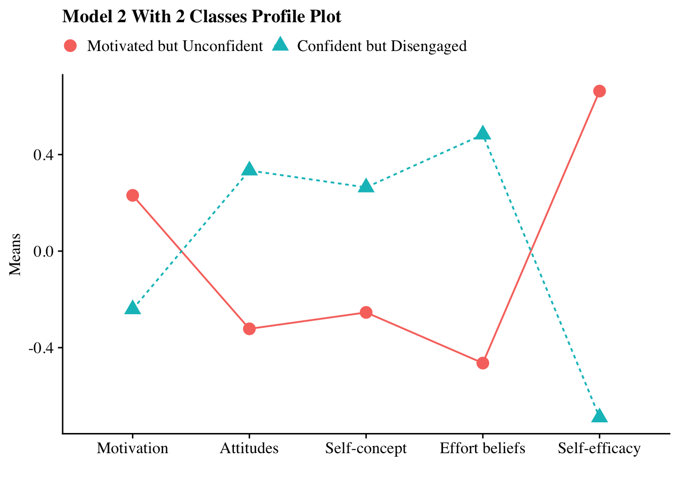

Final figure

plot_lpa <- function(model_name) {

  # Extract and reshape mean estimates by class
  pp_plots <- data.frame(model_name$parameters$unstandardized) %>%
    mutate(LatentClass = sub("^", "Class ", LatentClass)) %>%
    filter(paramHeader == "Means") %>%
    filter(LatentClass != "Class Categorical.Latent.Variables") %>%
    dplyr::select(est, LatentClass, param) %>%
    pivot_wider(names_from = LatentClass, values_from = est) %>%
    relocate(param, .after = last_col())
  
  # Extract class proportions
  c_size <- as.data.frame(model_name$class_counts$modelEstimated$proportion) %>%
    dplyr::rename("cs" = 1) %>%
    mutate(cs = round(cs * 100, 2))
  
  # Rename class labels with proportions
# Keep class labels without proportions
  colnames(pp_plots) <- c("Motivated but Unconfident", "Confident but Disengaged", "param")

  
  # Melt data into long format
  plot_data <- pp_plots %>%
    dplyr::rename("param" = ncol(pp_plots)) %>%
    reshape2::melt(id.vars = "param") %>%
    mutate(
     param = factor(param,
                   levels = c("Z_AMSC", "Z_ASCI_IA", "Z_CSC", "Z_EB", "Z_MSLQ"),
                   labels = c("Chemistry\nmotivation", "Chemistry\nattitudes", "Chemistry\nself-concept", "Effort beliefs", "Self-efficacy")),
     variable = factor(variable)
    )
  
  # Title
  name <- str_to_title(model_name$input$title)
  
  # Define color palette (can customize further)
  #class_colors <- c("#1b1b1b", "#595959", "#a6a6a6", "#d9d9d9")  # Extend if >2 classes
  class_colors <- c("#F8766D", "#005B96")  # red and dark blue
  
  # Plot
  p <- plot_data %>%
    ggplot(
      aes(
        x = param,
        y = value,
        shape = variable,
        colour = variable,
        lty = variable,
        group = variable
      )
    ) +
    geom_line(linewidth = 1) +
    geom_point(size = 4) +
    scale_x_discrete("") +
    scale_y_continuous(
    limits = c(-0.8, 0.8),
    breaks = c(-0.75, -0.5, -0.25, 0, 0.25, 0.5, 0.75)
    ) +
    scale_color_manual(values = class_colors[1:nlevels(plot_data$variable)]) +  # custom colors
    #labs(title = glue("{name} Profile Plot"), y = "Standardized indicator means") +
    labs(title = NULL, y = "Standardized indicator means") +
    theme_cowplot() +
    theme(
      text = element_text(family = "sans", size = 12),         # serif font
      axis.text = element_text(family = "sans", size = 12),    # axis labels
      axis.title = element_text(family = "sans", size = 14),    # axis labels
      legend.text = element_text(family = "sans", size = 12),  # legend text
      legend.title = element_text(family = "sans", size = 14),
      #legend.position = "top",
      legend.position = "none",
      panel.border = element_rect(colour = "black", fill = NA, linewidth = 1),
      axis.line = element_line(colour = "black", linewidth = 0.3)
    )
  
  return(p)
}

plot_lpa(model_name = output_pisa$model_2_class_2.out)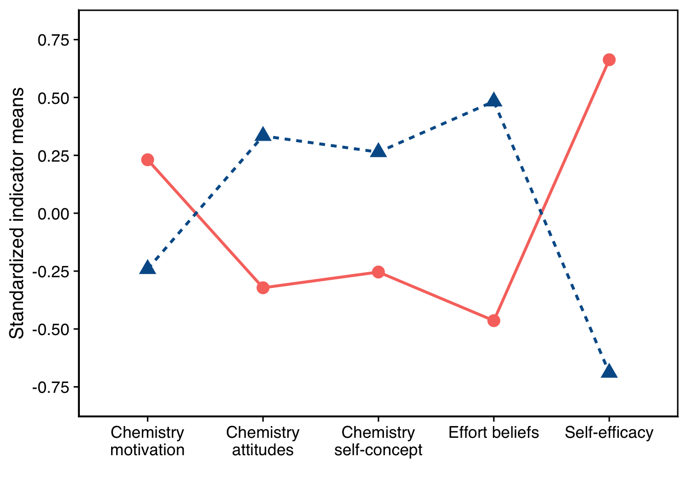


p <- plot_lpa(model_name = output_pisa$model_2_class_2.out)
ggsave("profile_plot.png", plot = p, width = 9, height = 5.6, units = "in", dpi = 600, bg = "white")

Three step ML

lpa_result <- pre_clean %>%
  dplyr::select(z_ASCI_IA, z_AMSC, z_EB, z_MSLQ, z_CSC) %>%
  estimate_profiles(n_profiles = 2, model = 2)  # Adjust the number of profiles as needed

classified_data <- bind_cols(pre_clean, get_data(lpa_result))

t.test(exam ~ Class, data = classified_data, var.equal = TRUE)
#> 
#>  Two Sample t-test
#> 
#> data:  exam by Class
#> t = 5.0593, df = 267, p-value = 7.837e-07
#> alternative hypothesis: true difference in means between group 1 and group 2 is not equal to 0
#> 95 percent confidence interval:
#>   5.064922 11.518549
#> sample estimates:
#> mean in group 1 mean in group 2 
#>        70.82609        62.53435

classified_data %>%
  group_by(Class) %>%
  summarise(
    n = n(),
    mean = mean(exam, na.rm = TRUE),
    sd = sd(exam, na.rm = TRUE)
  )
#> # A tibble: 2 × 4
#>   Class     n  mean    sd
#>   <dbl> <int> <dbl> <dbl>
#> 1     1   138  70.8  13.3
#> 2     2   131  62.5  13.6

wald test

lm_model <- lm(exam ~ Class, data = classified_data)
summary(lm_model)
#> 
#> Call:
#> lm(formula = exam ~ Class, data = classified_data)
#> 
#> Residuals:
#>     Min      1Q  Median      3Q     Max 
#> -30.826  -8.826   1.174   9.466  29.466 
#> 
#> Coefficients:
#>             Estimate Std. Error t value Pr(>|t|)    
#> (Intercept)   79.118      2.571  30.773  < 2e-16 ***
#> Class         -8.292      1.639  -5.059 7.84e-07 ***
#> ---
#> Signif. codes:  
#> 0 '***' 0.001 '**' 0.01 '*' 0.05 '.' 0.1 ' ' 1
#> 
#> Residual standard error: 13.44 on 267 degrees of freedom
#> Multiple R-squared:  0.08748,    Adjusted R-squared:  0.08406 
#> F-statistic:  25.6 on 1 and 267 DF,  p-value: 7.837e-07

Anova(lm_model, type = 3)  
#> Anova Table (Type III tests)
#> 
#> Response: exam
#>             Sum Sq  Df F value    Pr(>F)    
#> (Intercept) 170939   1 946.973 < 2.2e-16 ***
#> Class         4621   1  25.597 7.837e-07 ***
#> Residuals    48196 267                      
#> ---
#> Signif. codes:  
#> 0 '***' 0.001 '**' 0.01 '*' 0.05 '.' 0.1 ' ' 1

Kmeans

pre_clean <- pre_clean %>%
  mutate(across(all_of(c("ASCI_IA", "AMSC", "EB", "MSLQ", "CSC")), ~ scale(.)[,1], .names = "z_{.col}"))

dfk <- pre_clean %>%
  dplyr::select(z_ASCI_IA, z_AMSC, z_EB, z_MSLQ, z_CSC, exam, grading)

# Step 1: Select specific variables for clustering
dfk_selected <- dfk %>%
  dplyr::select(z_AMSC, z_ASCI_IA, z_CSC, z_EB, z_MSLQ) 

# Step 2: Scale the selected data
dfk_scaled <- scale(dfk_selected)

# Step 3: Set random seed for reproducibility
set.seed(123)

# Step 4: Run K-means for k = 2 to 10 and store total within-cluster sum of squares
wss <- numeric(9)
kmeans_results <- list()

for (k in 2:10) {
  km <- kmeans(dfk_scaled, centers = k, nstart = 10, iter.max = 25)
  wss[k - 1] <- km$tot.withinss
  kmeans_results[[as.character(k)]] <- km
}

# Step 5: Plot Elbow Method to choose optimal k
plot(2:10, wss, type = "b", pch = 19,
     xlab = "Number of Clusters (k)",
     ylab = "Total Within-Cluster Sum of Squares",
     main = "Elbow Method for Optimal k")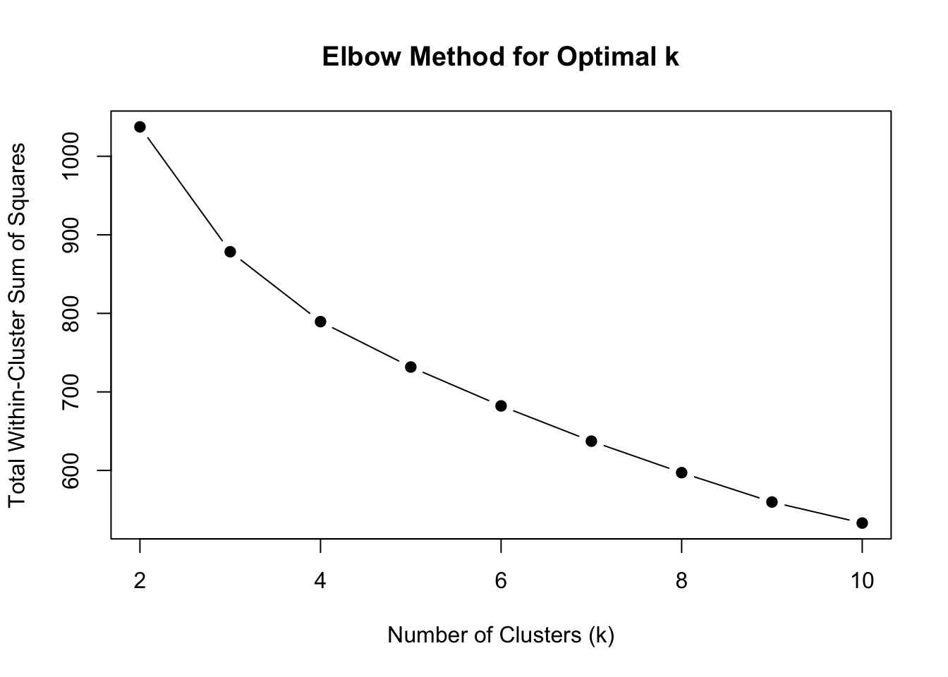


# Step 6: Assign cluster labels to the original selected data for chosen k
chosen_k <- 2
dfk_clustered <- dfk_selected %>%
  mutate(Cluster = factor(kmeans_results[[as.character(chosen_k)]]$cluster))

# Step 7: Visualize the clusters using PCA
fviz_cluster(kmeans_results[[as.character(chosen_k)]], data = dfk_scaled,
             geom = "point", ellipse.type = "convex",
             main = paste("K-means Clustering (k =", chosen_k, ")"))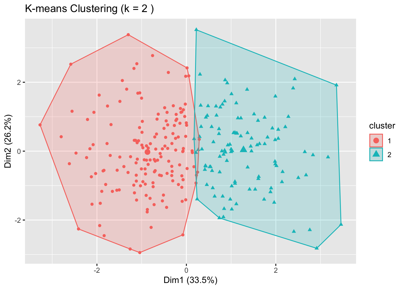

kmeans_results[["2"]]$size
#> [1] 160 109

fviz_nbclust(dfk_clustered, kmeans, method = "wss") #choose 3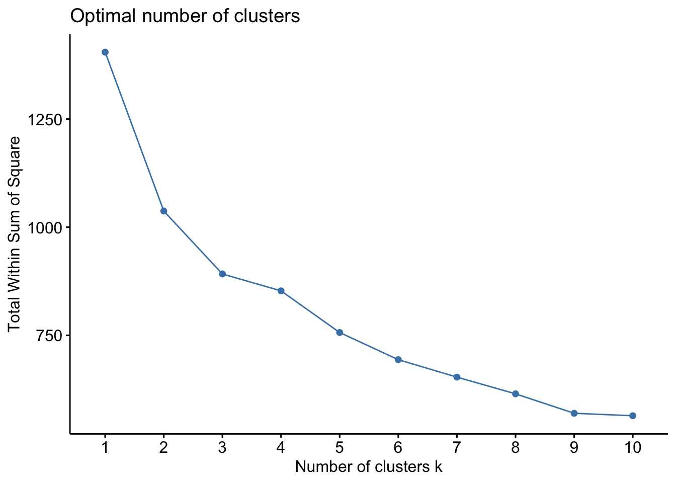

elbow plot

# Step 1: Add WSS for k = 1
# (Only if it wasn’t previously computed)
set.seed(123)
km1 <- kmeans(dfk_scaled, centers = 1, nstart = 10, iter.max = 25)
wss_full <- c(km1$tot.withinss, wss)  # Add k=1 to the front

# Step 2: Recreate full dataframe
elbow_df <- data.frame(
  k = 1:10,
  wss = wss_full
)

# Step 3: Create the updated plot
plot.wss <- ggplot(elbow_df, aes(x = k, y = wss)) +
  geom_line(color = "steelblue", linewidth = 1) +
  geom_point(color = "steelblue", size = 3) +
  scale_x_continuous(breaks = 1:10) +
  scale_y_continuous(limits = c(400, 1400)) +  # << Set y-axis range
  labs(
    x = expression("Number of clusters (" * italic(k) * ")"),
    y = "Total Within Sum of Squares (WSS)"
  ) +
  theme_minimal(base_size = 12) +
  theme(
    plot.title = element_blank(),
    panel.grid.major = element_blank(),
    panel.grid.minor = element_blank(),
    panel.border = element_rect(color = "black", fill = NA, linewidth = 1),
    axis.text = element_text(size = 12, color = "black"),
    axis.title = element_text(size = 14, color = "black"),
    axis.ticks.y = element_line(color = "black")
  )

plot.wss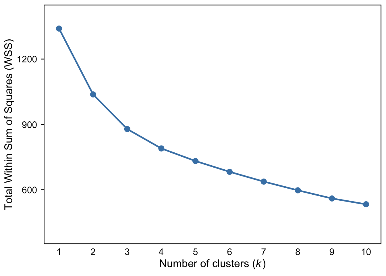


ggsave("cluster-wss.png", plot = plot.wss, width = 9, height = 5.6, units = "in", dpi = 600, bg = "white")

fviz_nbclust(dfk_clustered, kmeans, method = "silhouette") #choose 2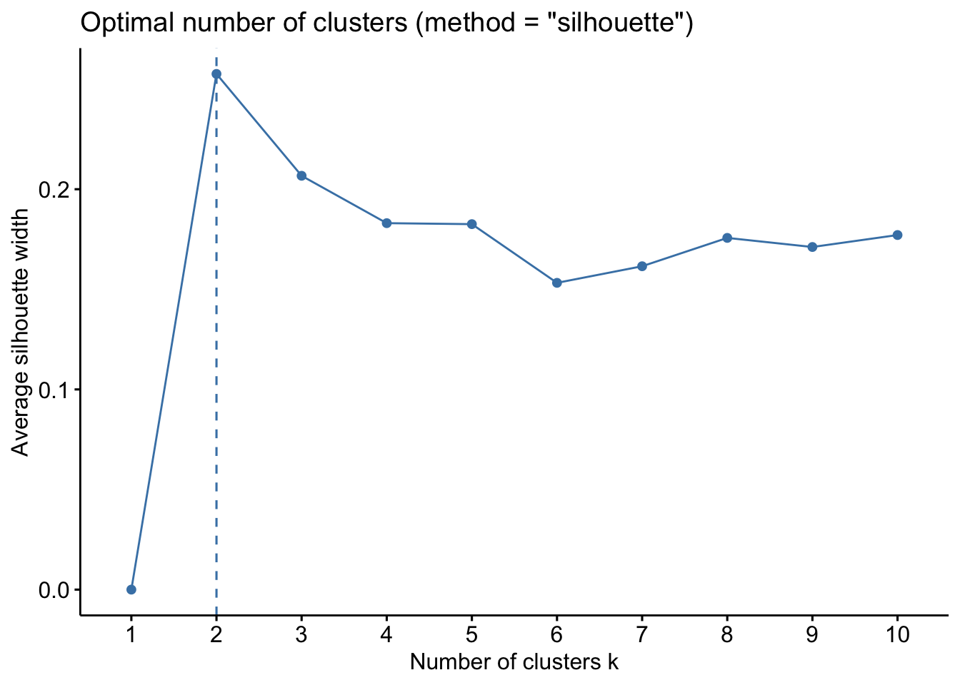


# Generate silhouette plot and customize it
plot.silhouette <- fviz_nbclust(dfk_clustered, kmeans, method = "silhouette") +
  geom_line(color = "steelblue", linewidth = 3) +
  geom_point(color = "steelblue", size = 3) +
  labs(
    x = expression("Number of clusters (" * italic(k) * ")"),
    y = "Average silhouette width",
    title = NULL
  ) +
  scale_x_discrete() +  # ← key fix here
  scale_y_continuous(limits = c(0, 0.3)) +
  theme_minimal(base_size = 12) +
  theme(
    panel.grid.major = element_blank(),
    panel.grid.minor = element_blank(),
    panel.border = element_rect(color = "black", fill = NA, linewidth = 1),
    axis.text = element_text(size = 12, color = "black"),
    axis.title = element_text(size = 14, color = "black"),
    axis.ticks.y = element_line(color = "black")
  )

plot.silhouette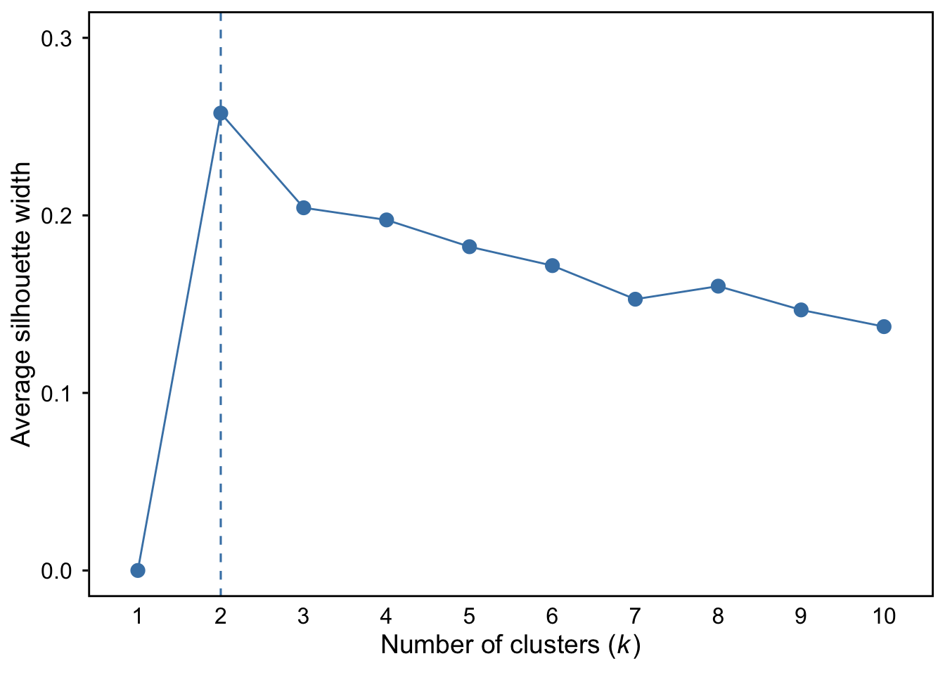


ggsave("silhouette.png", plot = plot.silhouette, width = 9, height = 5.6, units = "in", dpi = 600, bg = "white")

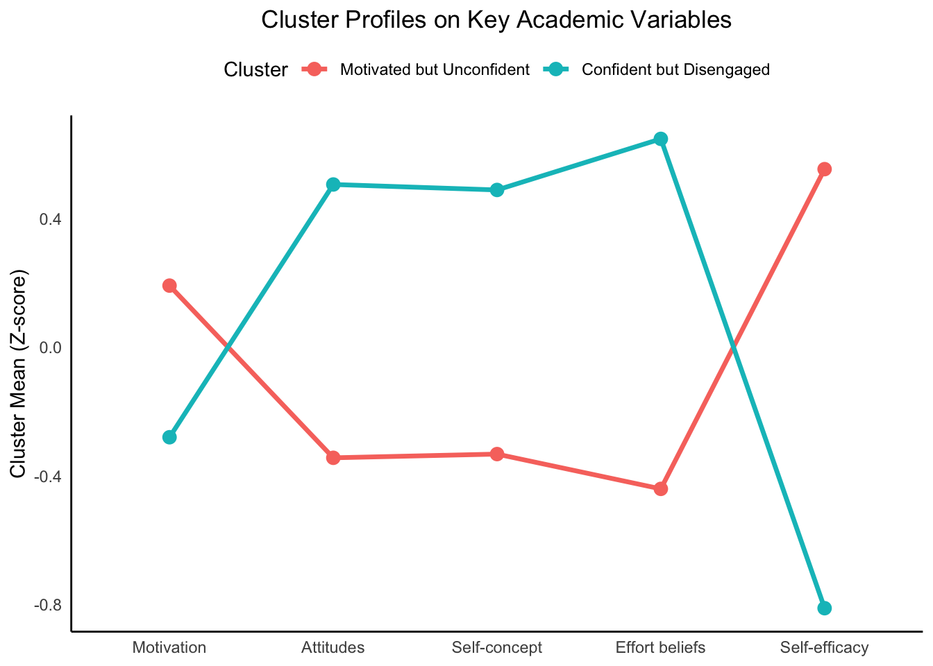
# Reshape the cluster centers data for plotting
long_data <- kmeans_results[["2"]]$centers %>%
  as.data.frame() %>%
  mutate(Cluster = factor(rownames(.))) %>%
  pivot_longer(-Cluster, names_to = "Variable", values_to = "Mean")

long_data$Cluster <- dplyr::recode(long_data$Cluster,
                            "1" = "Motivated but Unconfident",
                            "2" = "Confident but Disengaged")

# Define readable labels for each variable
variable_labels <- c("z_AMSC" = "Motivation",
                     "z_ASCI_IA" = "Attitudes",
                     "z_CSC" = "Self-concept",
                     "z_EB" = "Effort beliefs",
                     "z_MSLQ" = "Self-efficacy")

# Plot the cluster profiles
ggplot(long_data, aes(x = Variable, y = Mean, group = Cluster, color = Cluster)) +
  geom_line(linewidth = 1.2) +
  geom_point(size = 3) +
  theme_minimal() +
  labs(title = "Cluster Profiles on Key Academic Variables",
       y = "Cluster Mean (Z-score)",
       x = NULL) +
  scale_x_discrete(labels = variable_labels) +
  theme(
    axis.text.x = element_text(angle = 0, hjust = 0.5),  # Horizontal text
    plot.title = element_text(hjust = 0.5),
    legend.position = "top",
    legend.direction = "horizontal",
    panel.grid.major = element_blank(),  # remove major grid lines
    panel.grid.minor = element_blank(),   # remove minor grid lines
    axis.line.x = element_line(color = "black"),
    axis.line.y = element_line(color = "black")
  )

final cluster plot

# Define consistent color palette
cluster_colors <- c("Motivated but Unconfident" = "#F8766D",
                    "Confident but Disengaged" = "#005B96")

# Updated variable labels with line breaks
variable_labels <- c(
  "z_AMSC"    = "Chemistry\nmotivation",
  "z_ASCI_IA" = "Chemistry\nattitudes",
  "z_CSC"     = "Chemistry\nself-concept",
  "z_EB"      = "Effort beliefs",
  "z_MSLQ"    = "Self-efficacy"
)

# Generate the plot
plot.cluster <- ggplot(long_data, aes(x = Variable, y = Mean, group = Cluster, color = Cluster, linetype = Cluster, shape = Cluster)) +
  geom_line(linewidth = 1) +
  geom_point(size = 4) +
  scale_color_manual(values = cluster_colors) +
  scale_x_discrete(labels = variable_labels) +
  scale_y_continuous(
    limits = c(-0.9, 0.9),
    breaks = c(-0.75, -0.5, -0.25, 0, 0.25, 0.5, 0.75)
  ) +
  labs(
    #title = "Cluster Profiles on Key Academic Variables",
    y = "Standardized indicator means",
    x = NULL
  ) +
  theme_classic(base_family = "sans") +
  theme(
    text = element_text(size = 12),
    axis.text = element_text(size = 12, colour = "black"),
    axis.title = element_text(size = 14),
    legend.text = element_text(size = 12),
    legend.title = element_blank(),
    legend.position = "none",  # or "top" if you want to keep it
    panel.border = element_rect(colour = "black", fill = NA, linewidth = 0.8),
    axis.line = element_line(colour = "black", linewidth = 0.3)
  )

plot.cluster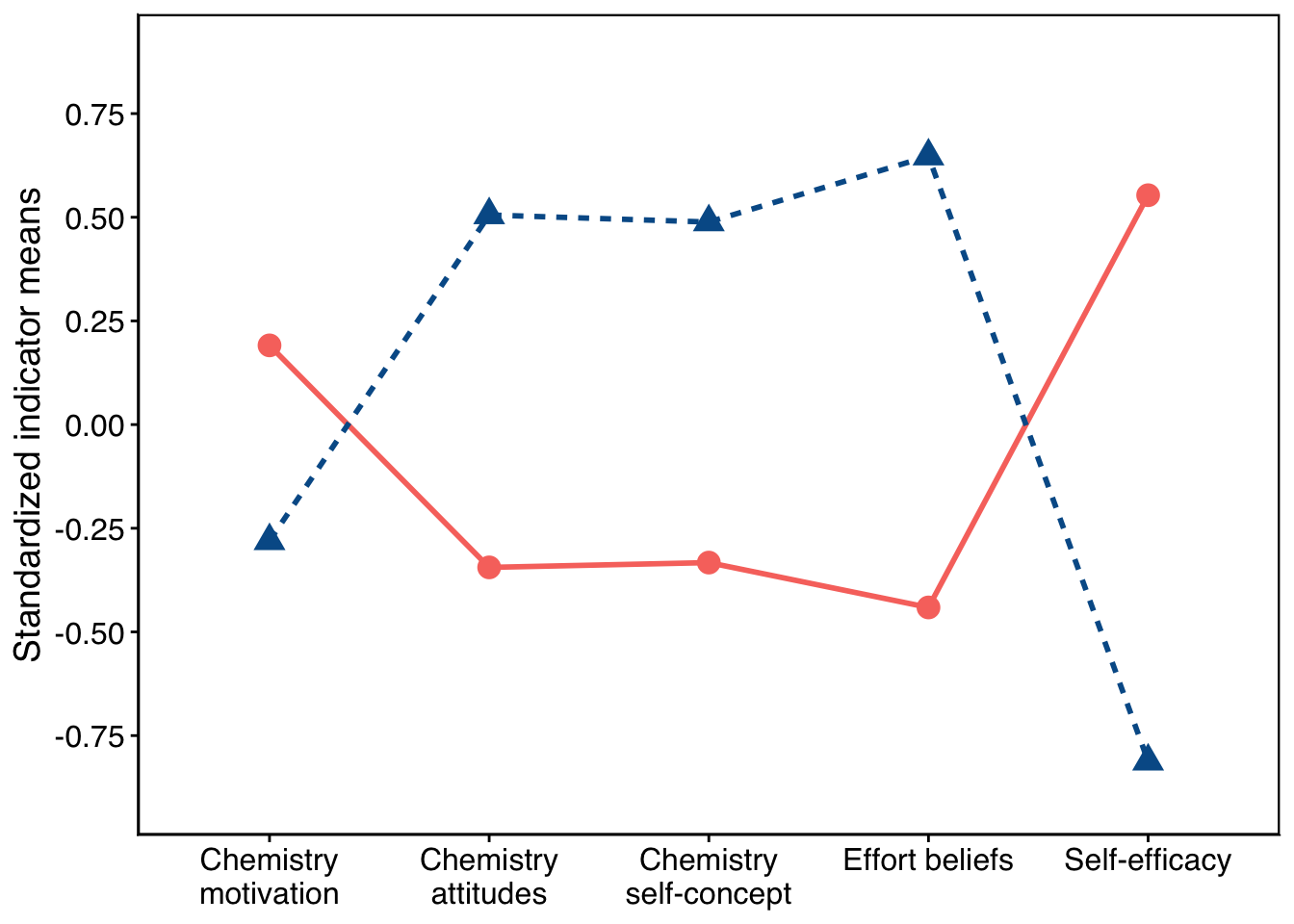


ggsave("cluster.png", plot = plot.cluster, width = 9, height = 5.6, units = "in", dpi = 600, bg = "white")

auxiliary

dfk_clustered <- dfk %>%
  dplyr::select(z_ASCI_IA, z_AMSC, z_EB, z_MSLQ, z_CSC, exam, grading) %>%  # include your two auxiliary variables
  drop_na() %>%  # drop rows with missing values
  mutate(Cluster = factor(kmeans_results[["2"]]$cluster))

# t-test for exam by Cluster (equal variances)
t.test(exam ~ Cluster, data = dfk_clustered, var.equal = TRUE)
#> 
#>  Two Sample t-test
#> 
#> data:  exam by Cluster
#> t = 4.664, df = 267, p-value = 4.906e-06
#> alternative hypothesis: true difference in means between group 1 and group 2 is not equal to 0
#> 95 percent confidence interval:
#>   4.52696 11.14116
#> sample estimates:
#> mean in group 1 mean in group 2 
#>        69.96250        62.12844

# t-test for grading by Cluster (equal variances)
t.test(grading ~ Cluster, data = dfk_clustered, var.equal = TRUE)
#> 
#>  Two Sample t-test
#> 
#> data:  grading by Cluster
#> t = -0.70234, df = 267, p-value = 0.4831
#> alternative hypothesis: true difference in means between group 1 and group 2 is not equal to 0
#> 95 percent confidence interval:
#>  -0.16508645  0.07827452
#> sample estimates:
#> mean in group 1 mean in group 2 
#>        0.543750        0.587156

dfk_clustered %>%
  group_by(Cluster) %>%
  summarise(
    Mean = mean(exam, na.rm = TRUE),
    SD = sd(exam, na.rm = TRUE),
    N = n()
  )
#> # A tibble: 2 × 4
#>   Cluster  Mean    SD     N
#>   <fct>   <dbl> <dbl> <int>
#> 1 1        70.0  13.4   160
#> 2 2        62.1  13.7   109

df_combined <- cbind(dfk_clustered, classified_data %>% rename(exam_2 = exam, grading_2 = grading))

tab <- df_combined %>%
  count(Cluster, Class) %>%
  group_by(Class) %>%
  mutate(percent = round(100 * n / sum(n), 1)) %>%
  ungroup()

tab <- tab %>%
  group_by(Class) %>%
  mutate(percent = round(100 * n / sum(n), 1)) %>%
  ungroup()

print(names(tab))
#> [1] "Cluster" "Class"   "n"       "percent"

tab %>%
  gt() %>%
  tab_header(
    title = "Contingency Table: K-means Cluster × LPA Class"
  ) %>%
  cols_label(
    Cluster = "K-means Cluster",
    Class = "LPA Class",
    n = "Count",
    percent = "Percent (%)"
  ) %>%
  fmt_number(columns = percent, decimals = 1)

K-means Cluster	LPA Class	Count	Percent (%)
Contingency Table: K-means Cluster × LPA Class
1	1	137	99.3
1	2	23	17.6
2	1	1	0.7
2	2	108	82.4

28 Math Attitudes with STEM Career Attainment (Dang, M., & Nylund-Gibson, K., 2017)

30 Moderation with a Latent Class Variable (Arch, Nylund-Gibson, Ing, 2026)