27 LTA with Measurement Invariance
27.1 Introduction
This R Markdown document accompanies the tutorial manuscript Latent Transition Analysis with Auxiliary Variables: A Demonstration of the ML 3-Step and BCH Methods in Mplus using data from the Longitudinal Study of American Youth (LSAY). Its purpose is to provide a fully reproducible, step-by-step implementation of the multi-step LTA workflow described in the paper using Mplus and the MplusAutomation package in R.
The focus of this document is operational rather than conceptual.
Before estimating the latent class structure, we begin by loading the necessary packages and preparing the dataset to ensure the indicators and sample structure are ready for LTA.
27.2 Data Setup and Preparation
27.2.1 Load Required Packages
# Installation required when using Mplus version 8.6
# devtools::install_github("michaelhallquist/MplusAutomation")
#if (!requireNamespace("BiocManager", quietly = TRUE))
# install.packages("BiocManager")
#BiocManager::install("rhdf5")

library(MplusAutomation)
library(rhdf5)
library(tidyverse)
library(haven)
library(here)
library(glue)
library(janitor)
library(gt)
library(naniar)
library(psych)
library(modelsummary)
library(cowplot)
library(patchwork)27.3 Descriptive Statistics
27.3.1 Indicators
# Define survey questions
all_questions <- c(
  "AB39A", "AB39H", "AB39I", "AB39K", "AB39L", "AB39M", "AB39T", "AB39U", "AB39W", "AB39X", # 7th grade
  "GA32A", "GA32H", "GA32I", "GA32K", "GA32L", "GA33A", "GA33H", "GA33I", "GA33K", "GA33L", # 10th grade
  "KA46A", "KA46H", "KA46I", "KA46K", "KA46L", "KA47A", "KA47H", "KA47I", "KA47K", "KA47L"  # 12th grade
)

# Function to compute stats (count, mean, SD, range)
compute_stats <- function(data, question, grade, question_name) {
  data %>%
    summarise(
      Grade = grade,
      Count = sum(!is.na(.data[[question]])),
      Mean = mean(.data[[question]], na.rm = TRUE),
      SD = sd(.data[[question]], na.rm = TRUE),
      Min = min(.data[[question]], na.rm = TRUE),
      Max = max(.data[[question]], na.rm = TRUE)
    ) %>%
    mutate(Question = question_name)
}

# Define question names and mappings
table_setup <- tibble(
  question_code = all_questions,
  grade = rep(c(7, 10, 12), each = 10),
  question_name = rep(
    c(
      "I enjoy math",
      "Math is useful in everyday problems",
      "Math helps a person think logically",
      "It is important to know math to get a good job",
      "I will use math in many ways as an adult",
      "I enjoy science",
      "Science is useful in everyday problems",
      "Science helps a person think logically",
      "It is important to know science to get a good job",
      "I will use science in many ways as an adult"
    ),
    times = 3
  )
)

# Compute stats for all questions
table1_data <- pmap_dfr(
  list(table_setup$question_code, table_setup$grade, table_setup$question_name),
  ~compute_stats(lsay_data, ..1, ..2, ..3)
) %>%
  mutate(
    Mean = round(Mean, 2),
    SD = round(SD, 2),
    Min = round(Min, 2),
    Max = round(Max, 2)
  ) %>%
  arrange(match(Question, table_setup$question_name), Grade) %>%
  select(Question, Grade, Count, Mean, SD, Min, Max)

# Build table
table1_gt <- table1_data %>%
  gt(groupname_col = "Question") %>%
  tab_header(
    title = "Table 1. Descriptive Statistics for Mathematics and Science Attitudinal Survey Items Included in Analyses"
  ) %>%
  cols_label(
    Grade = "Grade",
    Count = "N",
    Mean = "Prop.",
    SD = "SD",
    Min = "Min",
    Max = "Max"
  ) %>%
  fmt_number(
    columns = c(Mean, SD),
    decimals = 2
  )

# Show table
table1_gt| Table 1. Descriptive Statistics for Mathematics and Science Attitudinal Survey Items Included in Analyses | |||||
| Grade | N | Prop. | SD | Min | Max |
|---|---|---|---|---|---|
| I enjoy math | |||||
| 7 | 1882 | 0.69 | 0.46 | 0 | 1 |
| 10 | 1532 | 0.63 | 0.48 | 0 | 1 |
| 12 | 1120 | 0.57 | 0.50 | 0 | 1 |
| Math is useful in everyday problems | |||||
| 7 | 1851 | 0.72 | 0.45 | 0 | 1 |
| 10 | 1520 | 0.65 | 0.48 | 0 | 1 |
| 12 | 1111 | 0.67 | 0.47 | 0 | 1 |
| Math helps a person think logically | |||||
| 7 | 1847 | 0.65 | 0.48 | 0 | 1 |
| 10 | 1517 | 0.69 | 0.46 | 0 | 1 |
| 12 | 1108 | 0.71 | 0.45 | 0 | 1 |
| It is important to know math to get a good job | |||||
| 7 | 1854 | 0.77 | 0.42 | 0 | 1 |
| 10 | 1517 | 0.68 | 0.47 | 0 | 1 |
| 12 | 1105 | 0.61 | 0.49 | 0 | 1 |
| I will use math in many ways as an adult | |||||
| 7 | 1857 | 0.75 | 0.43 | 0 | 1 |
| 10 | 1525 | 0.65 | 0.48 | 0 | 1 |
| 12 | 1104 | 0.65 | 0.48 | 0 | 1 |
| I enjoy science | |||||
| 7 | 1873 | 0.62 | 0.48 | 0 | 1 |
| 10 | 1526 | 0.59 | 0.49 | 0 | 1 |
| 12 | 1105 | 0.55 | 0.50 | 0 | 1 |
| Science is useful in everyday problems | |||||
| 7 | 1840 | 0.40 | 0.49 | 0 | 1 |
| 10 | 1516 | 0.43 | 0.50 | 0 | 1 |
| 12 | 1099 | 0.48 | 0.50 | 0 | 1 |
| Science helps a person think logically | |||||
| 7 | 1850 | 0.49 | 0.50 | 0 | 1 |
| 10 | 1516 | 0.53 | 0.50 | 0 | 1 |
| 12 | 1100 | 0.56 | 0.50 | 0 | 1 |
| It is important to know science to get a good job | |||||
| 7 | 1857 | 0.40 | 0.49 | 0 | 1 |
| 10 | 1518 | 0.43 | 0.50 | 0 | 1 |
| 12 | 1099 | 0.38 | 0.49 | 0 | 1 |
| I will use science in many ways as an adult | |||||
| 7 | 1873 | 0.46 | 0.50 | 0 | 1 |
| 10 | 1524 | 0.42 | 0.49 | 0 | 1 |
| 12 | 1103 | 0.44 | 0.50 | 0 | 1 |
Data Verification Summary
All attitudinal indicators fall within the expected 0–1 range and show adequate variability across Grades 7, 10, and 12. No recoding or item removal is required before proceeding to enumeration.
27.3.2 Covariates
# Define covariates
covariates <- c(
  "MINORITY", "FEMALE"
)

# Function to compute stats (count, mean, SD, range, % missing)
compute_stats <- function(data, question, question_name) {
  total_n <- nrow(data)
  missing_n <- sum(is.na(data[[question]]))
  percent_missing <- (missing_n / total_n) * 100

  data %>%
    summarise(
      Count = sum(!is.na(.data[[question]])),
      Mean = mean(.data[[question]], na.rm = TRUE),
      SD = sd(.data[[question]], na.rm = TRUE),
      Min = min(.data[[question]], na.rm = TRUE),
      Max = max(.data[[question]], na.rm = TRUE)
    ) %>%
    mutate(
      Question = question_name,
      PercentMissing = round(percent_missing, 2)
    )
}

# Define question names and mappings
table_setup <- tibble(
  question_code = covariates,
  question_name = c(
    "Minority",
    "Gender"
  )
)

# Compute stats for all questions
table1_data <- pmap_dfr(
  list(table_setup$question_code, table_setup$question_name),
  ~compute_stats(lsay_data, ..1, ..2)
) %>%
  mutate(
    Mean = round(Mean, 2),
    SD = round(SD, 2),
    Min = round(Min, 2),
    Max = round(Max, 2)
  ) %>%
  select(Question, Count, PercentMissing, Mean, SD, Min, Max)

# Build table
table1_gt <- table1_data %>%
  gt() %>%
  tab_header(
    title = "Table 1. Descriptive Statistics for Covariates Included in Analyses"
  ) %>%
  cols_label(
    Count = "N",
    PercentMissing = "% Missing",
    Mean = "Mean or Proportion",
    SD = "SD",
    Min = "Min",
    Max = "Max"
  ) %>%
  fmt_number(
    columns = c(PercentMissing, Mean, SD, Min, Max),
    decimals = 2
  )

# Show table
table1_gt| Table 1. Descriptive Statistics for Covariates Included in Analyses | ||||||
| Question | N | % Missing | Mean or Proportion | SD | Min | Max |
|---|---|---|---|---|---|---|
| Minority | 1824 | 4.60 | 0.17 | 0.38 | 0.00 | 1.00 |
| Gender | 1912 | 0.00 | 0.51 | 0.50 | 0.00 | 1.00 |
Data Verification Summary
Covariates show valid ranges, expected missingness patterns, and sufficient variability for use in auxiliary-variable models. All covariates can be included as planned under full-information maximum likelihood.
27.4 Phase 1: Latent Class Enumeration at Each Timepoint (Exploratory Stage)
27.4.1 Time 1 Enumeration (Grade 7)
t1_enum <- lapply(1:6, function(k) {
  enum_t1  <- mplusObject(

   TITLE = glue("Class {k} Time 1"),

   VARIABLE = glue(
    "categorical = AB39A AB39H AB39I AB39K AB39L AB39M AB39T AB39U AB39W AB39X;
     usevar = AB39A AB39H AB39I AB39K AB39L AB39M AB39T AB39U AB39W AB39X;

     classes = c({k});"),

  ANALYSIS =
   "estimator = mlr;
    type = mixture;
    starts = 500 100;
    processors = 12;",

  OUTPUT = "sampstat residual tech11 tech14;",

  usevariables = colnames(lsay_data),
  rdata = lsay_data)

enum_t1_fit <- mplusModeler(enum_t1,
                 dataout=here("three_lta", "phase_1", "t1", "t1.dat"),
                 modelout=glue(here("three_lta", "phase_1", "t1", "c{k}_lca_t1.inp")),
                 check=TRUE, run = TRUE, hashfilename = FALSE)
})
27.4.2 Time 2 Enumeration (Grade 10)
t2_enum <- lapply(1:6, function(k) {
  enum_t2  <- mplusObject(

   TITLE = glue("Class {k} Time 2"),

   VARIABLE = glue(
    "categorical = GA32A GA32H GA32I GA32K GA32L GA33A GA33H GA33I GA33K GA33L;
     usevar = GA32A GA32H GA32I GA32K GA32L GA33A GA33H GA33I GA33K GA33L;

     classes = c({k});"),

  ANALYSIS =
   "estimator = mlr;
    type = mixture;
    starts = 500 100;
    processors = 12;",

  OUTPUT = "sampstat residual tech11 tech14;",

  usevariables = colnames(lsay_data),
  rdata = lsay_data)

enum_t2_fit <- mplusModeler(enum_t2,
                 dataout=here("three_lta", "phase_1", "t2", "t2.dat"),
                 modelout=glue(here("three_lta", "phase_1", "t2", "c{k}_lca_t2.inp")),
                 check=TRUE, run = TRUE, hashfilename = FALSE)
})
27.4.3 Time 3 Enumeration (Grade 12)
t3_enum <- lapply(1:6, function(k) {
  enum_t3  <- mplusObject(

   TITLE = glue("Class {k} Time 3"),

   VARIABLE = glue(
    "categorical = KA46A KA46H KA46I KA46K KA46L KA47A KA47H KA47I KA47K KA47L;
     usevar = KA46A KA46H KA46I KA46K KA46L KA47A KA47H KA47I KA47K KA47L;

     classes = c({k});"),

  ANALYSIS =
   "estimator = mlr;
    type = mixture;
    starts = 500 100;
    processors = 12;",

  OUTPUT = "sampstat residual tech11 tech14;",

  usevariables = colnames(lsay_data),
  rdata = lsay_data)

enum_t3_fit <- mplusModeler(enum_t3,
                 dataout=here("three_lta", "phase_1", "t3", "t3.dat"),
                 modelout=glue(here("three_lta", "phase_1", "t3", "c{k}_lca_t3.inp")),
                 check=TRUE, run = TRUE, hashfilename = FALSE)
})
Enumeration is completed for Grade 12. Agreement in class number and stability across all three waves provides initial empirical support for considering a longitudinal model.
27.5 Extracting and Summarizing Model Fit
27.5.1 Time 1
source(here("functions", "extract_mplus_info.R"))
source(here("functions","enum_table_lca.R"))

# Define the directory where all of the .out files are located.
output_dir <- here("three_lta", "phase_1","t1")

# Get all .out files
output_files <- list.files(output_dir, pattern = "\\.out$", full.names = TRUE)

# Process all .out files into one dataframe
final_data <- map_dfr(output_files, extract_mplus_info_extended)

# Extract Sample_Size from final_data
sample_size <- unique(final_data$Sample_Size)

output_enum_t1 <- readModels(here("three_lta", "phase_1","t1"), quiet = TRUE)
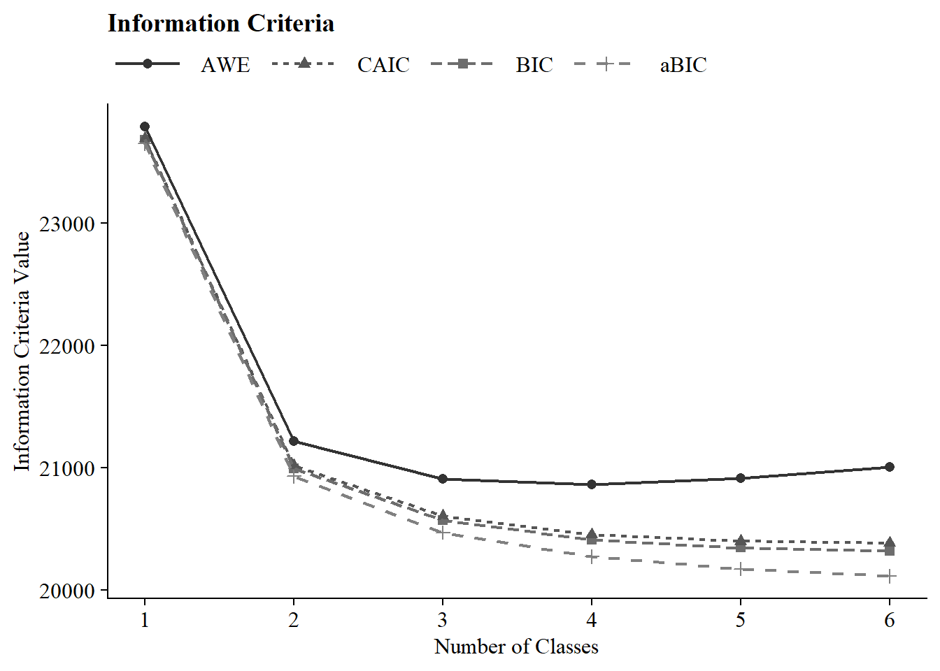
fit_table_lca(output_enum_t1, final_data)| Model Fit Summary Table1 | |||||||||||
| Classes | Par | LL | % Converged | % Replicated |
Model Fit Indices
|
LRTs
|
Smallest Class
|
||||
|---|---|---|---|---|---|---|---|---|---|---|---|
| BIC | aBIC | CAIC | AWE | VLMR | BLRT | n (%) | |||||
| Class 1 Time 1 | 10 | −11,803.43 | 100% | 100% | 23,682.28 | 23,650.51 | 23,692.28 | 23,787.70 | – | – | 1886 (100%) |
| Class 2 Time 1 | 21 | −10,418.76 | 100% | 100% | 20,995.91 | 20,929.19 | 21,016.91 | 21,217.29 | <.001 | <.001 | 782 (41.5%) |
| Class 3 Time 1 | 32 | −10,165.87 | 36% | 100% | 20,573.10 | 20,471.44 | 20,605.10 | 20,910.45 | 0.00 | <.001 | 384 (20.4%) |
| Class 4 Time 1 | 43 | −10,042.97 | 64% | 98% | 20,410.26 | 20,273.64 | 20,453.26 | 20,863.57 | 0.00 | <.001 | 390 (20.7%) |
| Class 5 Time 1 | 54 | −9,969.24 | 66% | 47% | 20,345.76 | 20,174.20 | 20,399.76 | 20,915.04 | 0.04 | <.001 | 175 (9.3%) |
| Class 6 Time 1 | 65 | −9,915.15 | 42% | 67% | 20,320.54 | 20,114.04 | 20,385.54 | 21,005.78 | 0.01 | <.001 | 180 (9.5%) |
| 1 Note. Par = Parameters; LL = model log likelihood; BIC = Bayesian information criterion; aBIC = sample size adjusted BIC; CAIC = consistent Akaike information criterion; AWE = approximate weight of evidence criterion; BLRT = bootstrapped likelihood ratio test p-value; VLMR = Vuong-Lo-Mendell-Rubin adjusted likelihood ratio test p-value; cmPk = approximate correct model probability. | |||||||||||
IC Plot
27.5.2 Time 2
# Define the directory where all of the .out files are located.
output_dir <- here("three_lta", "phase_1","t2")

# Get all .out files
output_files <- list.files(output_dir, pattern = "\\.out$", full.names = TRUE)

# Process all .out files into one dataframe
final_data <- map_dfr(output_files, extract_mplus_info_extended)

# Extract Sample_Size from final_data
sample_size <- unique(final_data$Sample_Size)

output_enum_t2 <- readModels(here("three_lta", "phase_1","t2"), quiet = TRUE)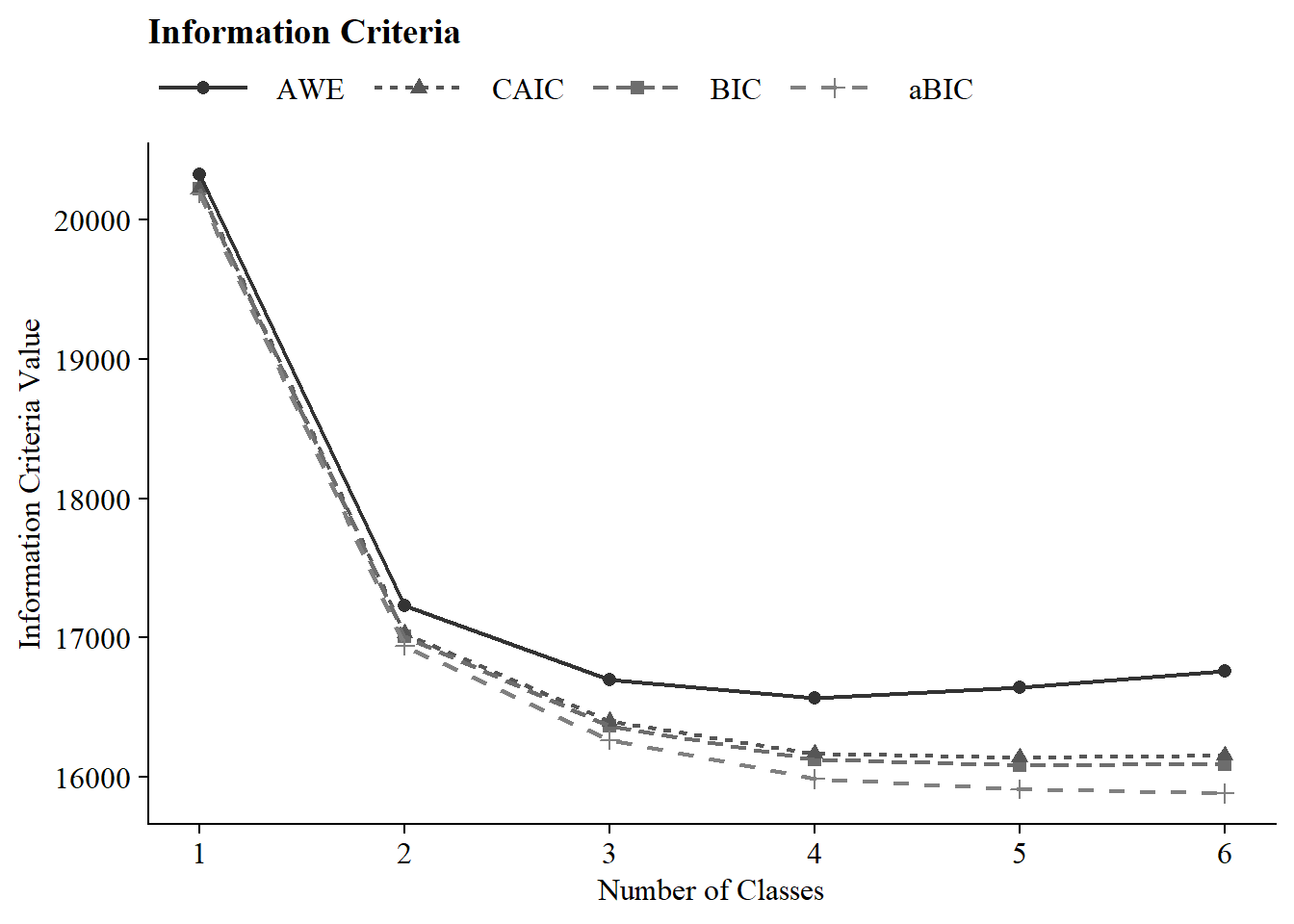
fit_table_lca(output_enum_t2, final_data)| Model Fit Summary Table1 | |||||||||||
| Classes | Par | LL | % Converged | % Replicated |
Model Fit Indices
|
LRTs
|
Smallest Class
|
||||
|---|---|---|---|---|---|---|---|---|---|---|---|
| BIC | aBIC | CAIC | AWE | VLMR | BLRT | n (%) | |||||
| Class 1 Time 2 | 10 | −10,072.93 | 100% | 100% | 20,219.21 | 20,187.44 | 20,229.21 | 20,322.56 | – | – | 1534 (100%) |
| Class 2 Time 2 | 21 | −8,428.38 | 100% | 100% | 17,010.82 | 16,944.10 | 17,031.82 | 17,227.86 | <.001 | <.001 | 658 (42.9%) |
| Class 3 Time 2 | 32 | −8,067.61 | 53% | 100% | 16,369.96 | 16,268.31 | 16,401.96 | 16,700.70 | <.001 | <.001 | 297 (19.4%) |
| Class 4 Time 2 | 43 | −7,905.53 | 39% | 100% | 16,126.50 | 15,989.90 | 16,169.50 | 16,570.93 | <.001 | <.001 | 290 (18.9%) |
| Class 5 Time 2 | 54 | −7,845.44 | 82% | 100% | 16,087.01 | 15,915.46 | 16,141.01 | 16,645.13 | 0.01 | <.001 | 220 (14.3%) |
| Class 6 Time 2 | 65 | −7,806.99 | 44% | 36% | 16,090.79 | 15,884.30 | 16,155.79 | 16,762.61 | 0.02 | <.001 | 130 (8.5%) |
| 1 Note. Par = Parameters; LL = model log likelihood; BIC = Bayesian information criterion; aBIC = sample size adjusted BIC; CAIC = consistent Akaike information criterion; AWE = approximate weight of evidence criterion; BLRT = bootstrapped likelihood ratio test p-value; VLMR = Vuong-Lo-Mendell-Rubin adjusted likelihood ratio test p-value; cmPk = approximate correct model probability. | |||||||||||
IC Plot
27.5.3 Time 3
# Define the directory where all of the .out files are located.
output_dir <- here("three_lta", "phase_1","t3")

# Get all .out files
output_files <- list.files(output_dir, pattern = "\\.out$", full.names = TRUE)

# Process all .out files into one dataframe
final_data <- map_dfr(output_files, extract_mplus_info_extended)

# Extract Sample_Size from final_data
sample_size <- unique(final_data$Sample_Size)

output_enum_t3 <- readModels(here("three_lta", "phase_1","t3"), quiet = TRUE)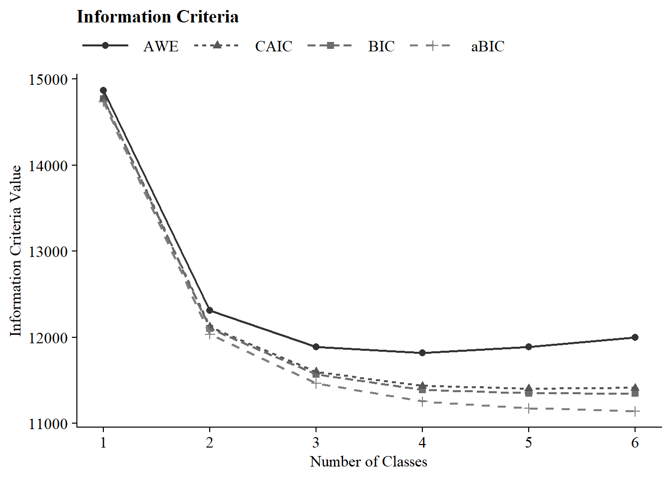
fit_table_lca(output_enum_t3, final_data)| Model Fit Summary Table1 | |||||||||||
| Classes | Par | LL | % Converged | % Replicated |
Model Fit Indices
|
LRTs
|
Smallest Class
|
||||
|---|---|---|---|---|---|---|---|---|---|---|---|
| BIC | aBIC | CAIC | AWE | VLMR | BLRT | n (%) | |||||
| Class 1 Time 3 | 10 | −7,349.13 | 100% | 100% | 14,768.49 | 14,736.72 | 14,778.49 | 14,868.72 | – | – | 1122 (100%) |
| Class 2 Time 3 | 21 | −5,976.60 | 100% | 100% | 12,100.68 | 12,033.98 | 12,121.68 | 12,311.16 | <.001 | <.001 | 534 (47.5%) |
| Class 3 Time 3 | 32 | −5,670.60 | 98% | 99% | 11,565.92 | 11,464.28 | 11,597.92 | 11,886.65 | <.001 | <.001 | 203 (18.1%) |
| Class 4 Time 3 | 43 | −5,543.62 | 36% | 97% | 11,389.22 | 11,252.64 | 11,432.22 | 11,820.20 | 0.00 | <.001 | 219 (19.5%) |
| Class 5 Time 3 | 54 | −5,483.67 | 63% | 62% | 11,346.57 | 11,175.06 | 11,400.57 | 11,887.81 | 0.00 | <.001 | 131 (11.7%) |
| Class 6 Time 3 | 65 | −5,444.06 | 42% | 64% | 11,344.60 | 11,138.14 | 11,409.60 | 11,996.08 | 0.09 | <.001 | 81 (7.2%) |
| 1 Note. Par = Parameters; LL = model log likelihood; BIC = Bayesian information criterion; aBIC = sample size adjusted BIC; CAIC = consistent Akaike information criterion; AWE = approximate weight of evidence criterion; BLRT = bootstrapped likelihood ratio test p-value; VLMR = Vuong-Lo-Mendell-Rubin adjusted likelihood ratio test p-value; cmPk = approximate correct model probability. | |||||||||||
IC Plot
27.6 1.5 Plotting Class Probabilities
Plot LCA:
source(here("functions","plot_lca.R"))

step1_t1 <- readModels(here("three_lta", "phase_1","t1"))
step1_t2 <- readModels(here("three_lta", "phase_1","t2"))
step1_t3 <- readModels(here("three_lta", "phase_1","t3"))

t1 <- step1_t1$c4_lca_t1.out
t2 <- step1_t2$c4_lca_t2.out
t3 <- step1_t3$c4_lca_t3.out


(plot_lca(t1) | plot_lca(t2) | plot_lca(t3))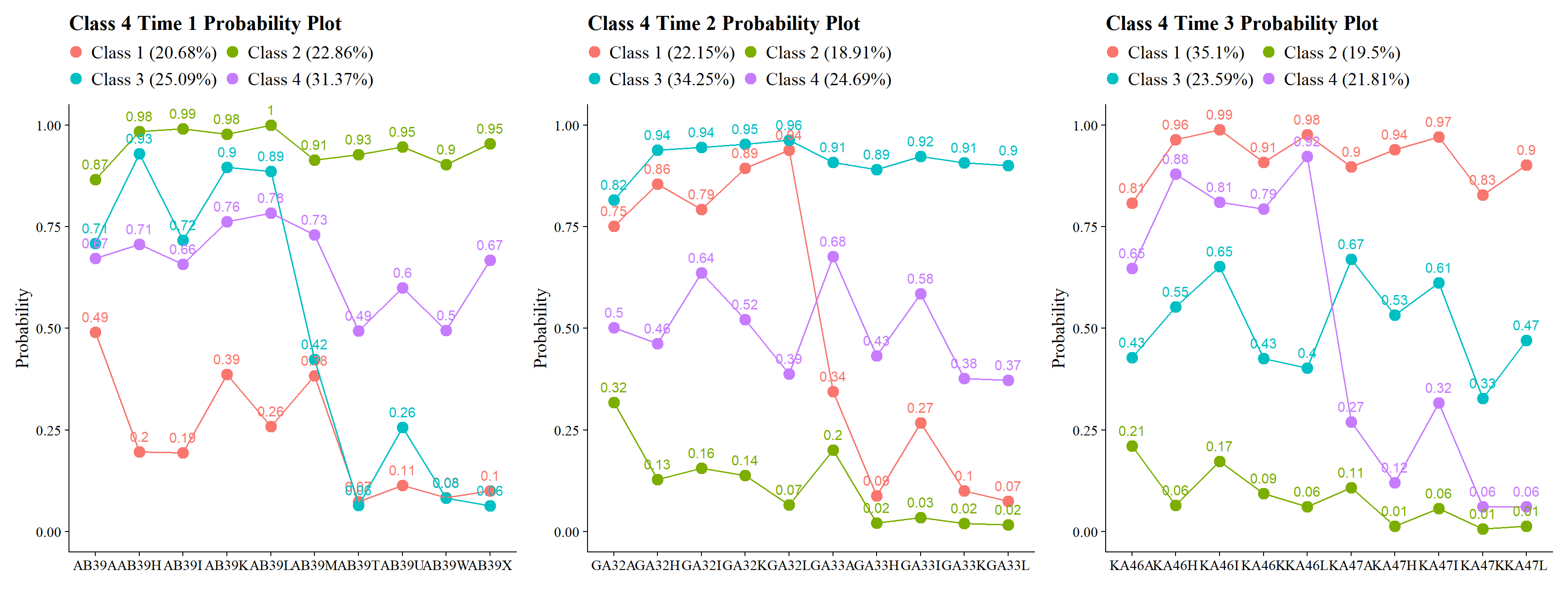
Class labels used here: Class 1: Very Positive, Class 2: Qualified Positive, Class 3: Neutral, Class 4: Less Positive
These diagnostics indicate that the same four-class structure is empirically recoverable across Grades 7, 10, and 12.
27.7 1.6 Estimate LCAs Independently at Each Time Point to Reorder Classes
In this step, the selected four-class solution is re-estimated independently at each wave with:
Fixed number of classes (four)
Optimized class ordering using
optseedSupplied
svalues()to enforce consistent class numbering across wavesRandom starts disabled (
starts = 0)
This step does not change the class structure. Its sole purpose is to ensure stable class labeling across waves prior to joint longitudinal modeling.
27.7.1 Time 1 (Reorder)
lca_t1  <- mplusObject(

  TITLE = "Class-3_Time1",

  VARIABLE =
   "categorical = AB39A AB39H AB39I AB39K AB39L AB39M AB39T AB39U AB39W AB39X;
         usevar = AB39A AB39H AB39I AB39K AB39L AB39M AB39T AB39U AB39W AB39X;
         !useobs = patw2==0;

    classes = c(4);",

  ANALYSIS =
   "estimator = mlr;
    type = mixture;
    starts = 0;
    optseed = 937588;",

  OUTPUT = "TECH1 TECH8 TECH14 svalues(2 3 4 1);",

  usevariables = colnames(lsay_data),
  rdata = lsay_data)


lca_t1_fit <- mplusModeler(lca_t1,
                 dataout=here("three_lta", "phase_1","reordered","t1_lca.dat"),
                 modelout=here("three_lta", "phase_1","reordered","t1_lca_step1.inp"),
                 check=TRUE, run = TRUE, hashfilename = FALSE)
27.7.2 Time 2 (Reorder)
lca_t2  <- mplusObject(

  TITLE = "Class-3_Time2",

  VARIABLE =
   "categorical = GA32A GA32H GA32I GA32K GA32L GA33A GA33H GA33I GA33K GA33L;
         usevar = GA32A GA32H GA32I GA32K GA32L GA33A GA33H GA33I GA33K GA33L;
         !useobs = patw4==0;

    classes = c(4);",

  ANALYSIS =
   "estimator = mlr;
    type = mixture;
    starts = 0;
    optseed = 264935;",

  OUTPUT = "TECH1 TECH8 TECH14 svalues(3 1 4 2);",

  usevariables = colnames(lsay_data),
  rdata = lsay_data)


lca_t2_fit <- mplusModeler(lca_t2,
                 dataout=here("three_lta", "phase_1","reordered","t2_lca.dat"),
                 modelout=here("three_lta", "phase_1","reordered","t2_lca_step1.inp"),
                 check=TRUE, run = TRUE, hashfilename = FALSE)
27.7.3 Time 3 (Reorder)
lca_t3  <- mplusObject(

  TITLE = "Class-3_Time3",

  VARIABLE =
   "categorical = KA46A KA46H KA46I KA46K KA46L KA47A KA47H KA47I KA47K KA47L;
         usevar = KA46A KA46H KA46I KA46K KA46L KA47A KA47H KA47I KA47K KA47L;
         !useobs = patw6==0;

    classes = c(4);",

  ANALYSIS =
   "estimator = mlr;
    type = mixture;
    starts = 0;
    optseed = 366706;",

  OUTPUT = "TECH1 TECH8 TECH14 svalues(1 4 3 2);",

  usevariables = colnames(lsay_data),
  rdata = lsay_data)


lca_t3_fit <- mplusModeler(lca_t3,
                 dataout=here("three_lta", "phase_1","reordered","t3_lca.dat"),
                 modelout=here("three_lta", "phase_1","reordered","t3_lca_step1.inp"),
                 check=TRUE, run = TRUE, hashfilename = FALSE)
27.7.4 Diagnostic Class Plots (Post-Reordering)
source(here("functions","plot_lca.R"))
t1 <- readModels(here("three_lta", "phase_1","reordered","t1_lca_step1.out"))
t2 <- readModels(here("three_lta", "phase_1","reordered","t2_lca_step1.out"))
t3 <- readModels(here("three_lta", "phase_1","reordered","t3_lca_step1.out"))


(plot_lca(t1) | plot_lca(t2) | plot_lca(t3))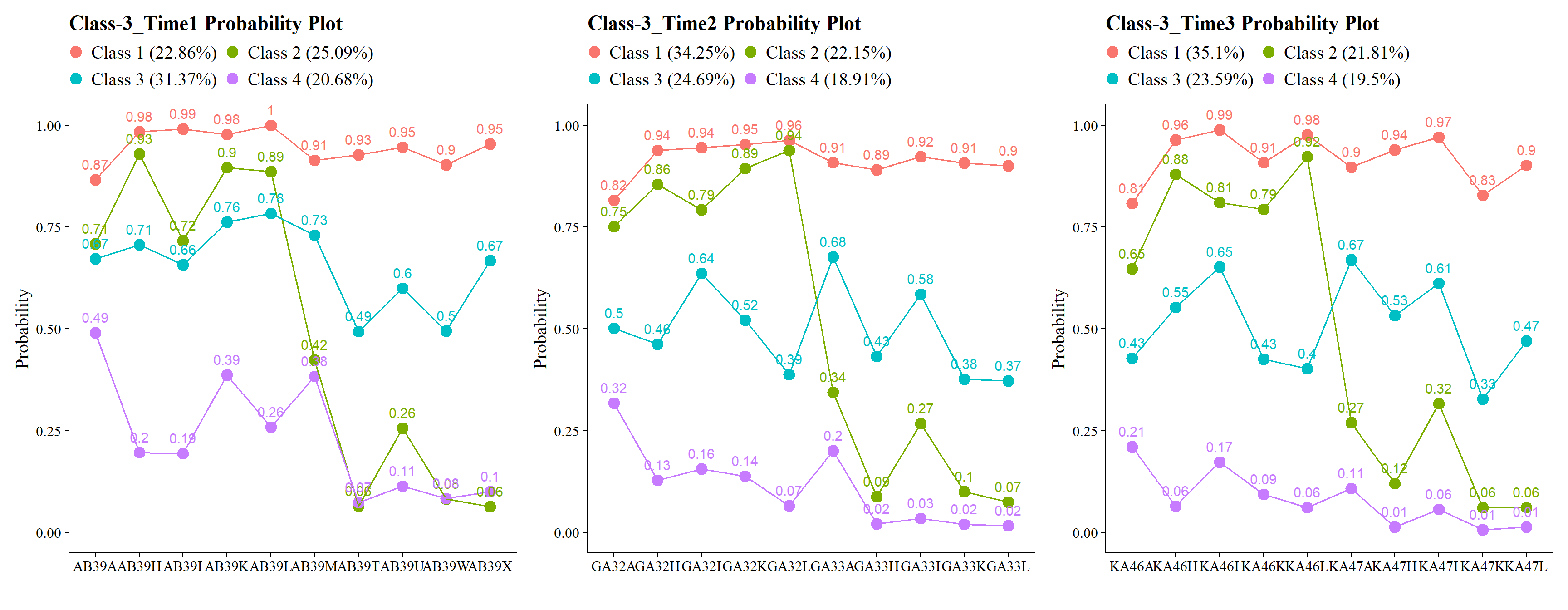
27.8 Phase 2: Testing for Measurement Invariance
27.8.1 Estimate the Non-Invariant Joint Configural Model (No Transitions)
lta_non_inv <- mplusObject(

  TITLE =
    "Non-Invariant LTA Model",

  VARIABLE =
     "idvariable=CASENUM;

      usev =
      AB39A AB39H AB39I AB39K AB39L AB39M AB39T AB39U AB39W AB39X
      GA32A GA32H GA32I GA32K GA32L GA33A GA33H GA33I GA33K GA33L
      KA46A KA46H KA46I KA46K KA46L KA47A KA47H KA47I KA47K KA47L;

      categorical =
      AB39A AB39H AB39I AB39K AB39L AB39M AB39T AB39U AB39W AB39X
      GA32A GA32H GA32I GA32K GA32L GA33A GA33H GA33I GA33K GA33L
      KA46A KA46H KA46I KA46K KA46L KA47A KA47H KA47I KA47K KA47L;

      classes = c1(4) c2(4) c3(4);",

  ANALYSIS =
     "estimator = mlr;
      type = mixture;
      starts = 500 200;",

  MODEL =
     "%overall%

  MODEL c1:
     %c1#1%
     [AB39A$1-AB39X$1];
     %c1#2%
     [AB39A$1-AB39X$1];
     %c1#3%
     [AB39A$1-AB39X$1];
     %c1#4%
     [AB39A$1-AB39X$1];

  MODEL c2:
     %c2#1%
     [GA32A$1-GA33L$1];
     %c2#2%
     [GA32A$1-GA33L$1];
     %c2#3%
     [GA32A$1-GA33L$1];
     %c2#4%
     [GA32A$1-GA33L$1];

  MODEL c3:
     %c3#1%
     [KA46A$1-KA47L$1];
     %c3#2%
     [KA46A$1-KA47L$1];
     %c3#3%
     [KA46A$1-KA47L$1];
     %c3#4%
     [KA46A$1-KA47L$1];",

  OUTPUT = "svalues;",

  usevariables = colnames(lsay_data),
  rdata = lsay_data)

lta_non_inv_fit <- mplusModeler(lta_non_inv,
                     dataout=here("three_lta", "phase_2", "lta.dat"),
                     modelout=here("three_lta", "phase_2", "noninvariant_lta.inp"),
                     check=TRUE, run = TRUE, hashfilename = FALSE)
After estimation, this model is retained strictly as the reference model for nested testing.
27.8.2 Estimate the Full Measurement-Invariance Model
lta_inv <- mplusObject(

  TITLE =
    "Invariant LTA Model",

  VARIABLE =
     "idvariable=CASENUM;

      usev =
      AB39A AB39H AB39I AB39K AB39L AB39M AB39T AB39U AB39W AB39X
      GA32A GA32H GA32I GA32K GA32L GA33A GA33H GA33I GA33K GA33L
      KA46A KA46H KA46I KA46K KA46L KA47A KA47H KA47I KA47K KA47L;

      categorical =
      AB39A AB39H AB39I AB39K AB39L AB39M AB39T AB39U AB39W AB39X
      GA32A GA32H GA32I GA32K GA32L GA33A GA33H GA33I GA33K GA33L
      KA46A KA46H KA46I KA46K KA46L KA47A KA47H KA47I KA47K KA47L;

      classes = c1(4) c2(4) c3(4);",

  ANALYSIS =
     "estimator = mlr;
      type = mixture;
      starts =  0;
      processors=10;",

  MODEL =
     "
     %overall%

  MODEL c1:
     %c1#1%
     [AB39A$1-AB39X$1](1-10);
     %c1#2%
     [AB39A$1-AB39X$1](11-20);
     %c1#3%
     [AB39A$1-AB39X$1](21-30);
     %c1#4%
     [AB39A$1-AB39X$1](31-40);

  MODEL c2:
     %c2#1%
     [GA32A$1-GA33L$1](1-10);
     %c2#2%
     [GA32A$1-GA33L$1](11-20);
     %c2#3%
     [GA32A$1-GA33L$1](21-30);
     %c2#4%
     [GA32A$1-GA33L$1](31-40);

  MODEL c3:
     %c3#1%
     [KA46A$1-KA47L$1](1-10);
     %c3#2%
     [KA46A$1-KA47L$1](11-20);
     %c3#3%
     [KA46A$1-KA47L$1](21-30);
     %c3#4%
     [KA46A$1-KA47L$1](31-40);",

  OUTPUT = "svalues;",

  usevariables = colnames(lsay_data),
  rdata = lsay_data)

lta_inv_fit <- mplusModeler(lta_inv,
                     dataout=here("three_lta", "phase_2", "lta.dat"),
                     modelout=here("three_lta", "phase_2", "invariant_lta.inp"),
                     check=TRUE, run = TRUE, hashfilename = FALSE)
This model yields the measurement structure used for all downstream auxiliary-variable analyses if invariance is retained.
27.8.3 Plotting the Non-Invariant and Invariant Models
source(here("functions","plot_lta.R"))

inv_mod <- readModels(here("three_lta", "phase_2"), quiet = TRUE)

plot_lta(inv_mod$invariant_lta.out)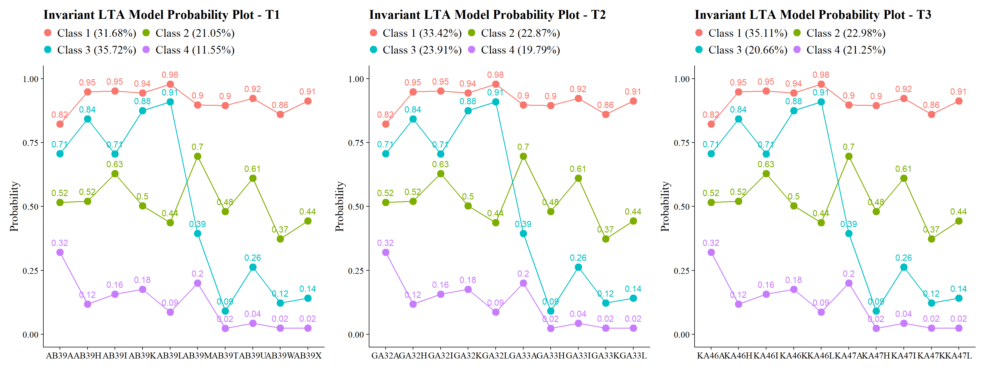
plot_lta(inv_mod$noninvariant_lta.out)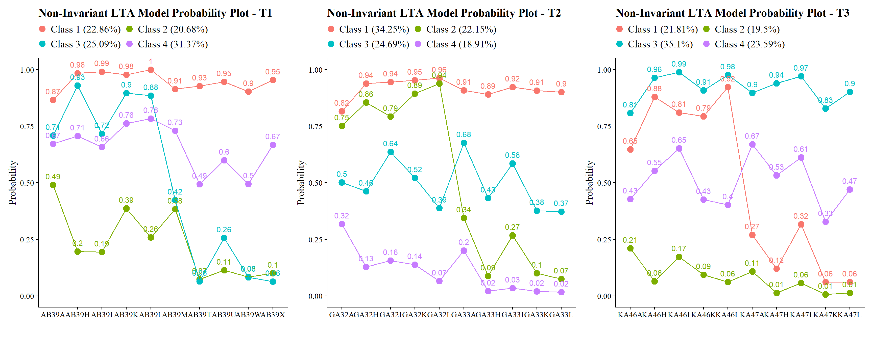
27.9 Nested Model Testing: Satorra–Bentler Scaled χ² Difference Test
# *0 = null or nested model & *1 = comparison  or parent model
lta_models <- readModels(here("three_lta", "phase_2"), quiet = TRUE)

# Log Likelihood Values
L0 <- lta_models$invariant_lta.out$summaries$LL
L1 <- lta_models$noninvariant_lta.out$summaries$LL

# LRT equation
lr <- -2*(L0-L1)

# Parameters
p0 <- lta_models$invariant_lta.out$summaries$Parameters
p1 <- lta_models$noninvariant_lta.out$summaries$Parameters

# Scaling Correction Factors
c0 <- lta_models$invariant_lta.out$summaries$LLCorrectionFactor
c1 <- lta_models$noninvariant_lta.out$summaries$LLCorrectionFactor

# Difference Test Scaling correction
cd <- ((p0*c0)-(p1*c1))/(p0-p1)

# Chi-square difference test(TRd)
TRd <- (lr)/(cd)

# Degrees of freedom
df <- abs(p0 - p1)

# Significance test
(p_diff <- pchisq(TRd, df, lower.tail=FALSE))
#> [1] 2.294394e-40
27.10 Alternatively: Nested Model Testing Using compareModels in MplusAutomation
invisible(capture.output(
  comparison <- compareModels(lta_models$invariant_lta.out, lta_models$noninvariant_lta.out, diffTest=TRUE)
))

# p-value
comparison$diffTest$MLR_LL$p
#> [1] 2.294394e-40

#BIC
comparison$summaries
#>                     Title Observations Estimator Parameters
#> 1     Invariant LTA Model         1907       MLR         49
#> 2 Non-Invariant LTA Model         1907       MLR        129
#>          LL      AIC      BIC
#> 1 -23700.74 47499.48 47771.59
#> 2 -23492.12 47242.24 47958.6227.12 ML Three-Step Procedure
27.12.1 ML STEP 1: Re-Estimate
Time 1: Fixed-Threshold LCA With Saved CPROBS
inv_t1  <- mplusObject(

  TITLE = "Time 1 - Invariant LCA",

  VARIABLE =
   "idvariable=CASENUM;
    categorical = AB39A AB39H AB39I AB39K AB39L AB39M AB39T AB39U AB39W AB39X;
         usevar = AB39A AB39H AB39I AB39K AB39L AB39M AB39T AB39U AB39W AB39X;

    classes = c1(4);

    auxiliary = MINORITY, FEMALE, MATHG7, MATHG10, MATHG12;",

  ANALYSIS =
   "estimator = mlr;
    type = mixture;
    starts = 0;",

  MODEL =
     "%overall%

     %C1#1%

     [ ab39a$1@-1.53313 ] (1);
     [ ab39h$1@-2.90401 ] (2);
     [ ab39i$1@-2.99575 ] (3);
     [ ab39k$1@-2.83359 ] (4);
     [ ab39l$1@-3.85594 ] (5);
     [ ab39m$1@-2.16372 ] (6);
     [ ab39t$1@-2.13876 ] (7);
     [ ab39u$1@-2.48348 ] (8);
     [ ab39w$1@-1.81515 ] (9);
     [ ab39x$1@-2.35163 ] (10);

     %C1#3%

     [ ab39a$1@-0.06349 ] (11);
     [ ab39h$1@-0.07976 ] (12);
     [ ab39i$1@-0.52495 ] (13);
     [ ab39k$1@-0.01216 ] (14);
     [ ab39l$1@0.25484 ] (15);
     [ ab39m$1@-0.83350 ] (16);
     [ ab39t$1@0.07961 ] (17);
     [ ab39u$1@-0.45274 ] (18);
     [ ab39w$1@0.51840 ] (19);
     [ ab39x$1@0.22569 ] (20);

     %C1#2%

     [ ab39a$1@-0.88292 ] (21);
     [ ab39h$1@-1.67761 ] (22);
     [ ab39i$1@-0.87642 ] (23);
     [ ab39k$1@-1.94409 ] (24);
     [ ab39l$1@-2.31259 ] (25);
     [ ab39m$1@0.42887 ] (26);
     [ ab39t$1@2.29606 ] (27);
     [ ab39u$1@1.02908 ] (28);
     [ ab39w$1@1.97179 ] (29);
     [ ab39x$1@1.80988 ] (30);

     %C1#4%

     [ ab39a$1@0.74744 ] (31);
     [ ab39h$1@2.01287 ] (32);
     [ ab39i$1@1.67957 ] (33);
     [ ab39k$1@1.54221 ] (34);
     [ ab39l$1@2.34965 ] (35);
     [ ab39m$1@1.38217 ] (36);
     [ ab39t$1@3.73153 ] (37);
     [ ab39u$1@3.09927 ] (38);
     [ ab39w$1@3.69495 ] (39);
     [ ab39x$1@3.68803 ] (40);",

  OUTPUT = "TECH1 TECH8 TECH14;",

  SAVEDATA =
   "File=t1_inv_cprobs.dat;
    Save=cprob;",

  usevariables = colnames(lsay_data),
  rdata = lsay_data)


inv_t1_fit <- mplusModeler(inv_t1,
                 dataout=here("three_lta", "phase_3","step_1_ml", "t1_inv.dat"),
                 modelout=here("three_lta", "phase_3","step_1_ml", "t1_inv_lca.inp"),
                 check=TRUE, run = TRUE, hashfilename = FALSE)
Time 2: Fixed-Threshold LCA With Saved CPROBS
inv_t2  <- mplusObject(

  TITLE = "Time 2 - Invariant LCA",

  VARIABLE =
   "idvariable=CASENUM;
    categorical = GA32A GA32H GA32I GA32K GA32L GA33A GA33H GA33I GA33K GA33L;
         usevar = GA32A GA32H GA32I GA32K GA32L GA33A GA33H GA33I GA33K GA33L;

    classes = c2(4);

    auxiliary = MINORITY, FEMALE, MATHG7, MATHG10, MATHG12;",

  ANALYSIS =
   "estimator = mlr;
    type = mixture;
    starts = 0;",

  MODEL =
     "%overall%

     %C2#1%

     [ ga32a$1@-1.53313 ] (1);
     [ ga32h$1@-2.90401 ] (2);
     [ ga32i$1@-2.99575 ] (3);
     [ ga32k$1@-2.83359 ] (4);
     [ ga32l$1@-3.85594 ] (5);
     [ ga33a$1@-2.16372 ] (6);
     [ ga33h$1@-2.13876 ] (7);
     [ ga33i$1@-2.48348 ] (8);
     [ ga33k$1@-1.81515 ] (9);
     [ ga33l$1@-2.35163 ] (10);

     %C2#3%

     [ ga32a$1@-0.06349 ] (11);
     [ ga32h$1@-0.07976 ] (12);
     [ ga32i$1@-0.52495 ] (13);
     [ ga32k$1@-0.01216 ] (14);
     [ ga32l$1@0.25484 ] (15);
     [ ga33a$1@-0.83350 ] (16);
     [ ga33h$1@0.07961 ] (17);
     [ ga33i$1@-0.45274 ] (18);
     [ ga33k$1@0.51840 ] (19);
     [ ga33l$1@0.22569 ] (20);

     %C2#2%

     [ ga32a$1@-0.88292 ] (21);
     [ ga32h$1@-1.67761 ] (22);
     [ ga32i$1@-0.87642 ] (23);
     [ ga32k$1@-1.94409 ] (24);
     [ ga32l$1@-2.31259 ] (25);
     [ ga33a$1@0.42887 ] (26);
     [ ga33h$1@2.29606 ] (27);
     [ ga33i$1@1.02908 ] (28);
     [ ga33k$1@1.97179 ] (29);
     [ ga33l$1@1.80988 ] (30);

     %C2#4%

     [ ga32a$1@0.74744 ] (31);
     [ ga32h$1@2.01287 ] (32);
     [ ga32i$1@1.67957 ] (33);
     [ ga32k$1@1.54221 ] (34);
     [ ga32l$1@2.34965 ] (35);
     [ ga33a$1@1.38217 ] (36);
     [ ga33h$1@3.73153 ] (37);
     [ ga33i$1@3.09927 ] (38);
     [ ga33k$1@3.69495 ] (39);
     [ ga33l$1@3.68803 ] (40);
",

  OUTPUT = "TECH1 TECH8 TECH14;",

  SAVEDATA =
   "File=t2_inv_cprobs.dat;
    Save=cprob;",

  usevariables = colnames(lsay_data),
  rdata = lsay_data)


inv_t2_fit <- mplusModeler(inv_t2,
                 dataout=here("three_lta", "phase_3","step_1_ml", "t2_inv.dat"),
                 modelout=here("three_lta", "phase_3","step_1_ml", "t2_inv_lca.inp"),
                 check=TRUE, run = TRUE, hashfilename = FALSE)
Time 3: Fixed-Threshold LCA With Saved CPROBS
inv_t3  <- mplusObject(

  TITLE = "Time 3 - Invariant LCA",

  VARIABLE =
   "idvariable=CASENUM;
    categorical = KA46A KA46H KA46I KA46K KA46L KA47A KA47H KA47I KA47K KA47L;
         usevar = KA46A KA46H KA46I KA46K KA46L KA47A KA47H KA47I KA47K KA47L;

    classes = c3(4);

    auxiliary = MINORITY, FEMALE, MATHG7, MATHG10, MATHG12;",

  ANALYSIS =
   "estimator = mlr;
    type = mixture;
    starts = 0;   ",

    MODEL =
     "%overall%

     %C3#1%

     [ ka46a$1@-1.53313 ] (1);
     [ ka46h$1@-2.90401 ] (2);
     [ ka46i$1@-2.99575 ] (3);
     [ ka46k$1@-2.83359 ] (4);
     [ ka46l$1@-3.85594 ] (5);
     [ ka47a$1@-2.16372 ] (6);
     [ ka47h$1@-2.13876 ] (7);
     [ ka47i$1@-2.48348 ] (8);
     [ ka47k$1@-1.81515 ] (9);
     [ ka47l$1@-2.35163 ] (10);

     %C3#2%

     [ ka46a$1@-0.06349 ] (11);
     [ ka46h$1@-0.07976 ] (12);
     [ ka46i$1@-0.52495 ] (13);
     [ ka46k$1@-0.01216 ] (14);
     [ ka46l$1@0.25484 ] (15);
     [ ka47a$1@-0.83350 ] (16);
     [ ka47h$1@0.07961 ] (17);
     [ ka47i$1@-0.45274 ] (18);
     [ ka47k$1@0.51840 ] (19);
     [ ka47l$1@0.22569 ] (20);

     %C3#3%

     [ ka46a$1@-0.88292 ] (21);
     [ ka46h$1@-1.67761 ] (22);
     [ ka46i$1@-0.87642 ] (23);
     [ ka46k$1@-1.94409 ] (24);
     [ ka46l$1@-2.31259 ] (25);
     [ ka47a$1@0.42887 ] (26);
     [ ka47h$1@2.29606 ] (27);
     [ ka47i$1@1.02908 ] (28);
     [ ka47k$1@1.97179 ] (29);
     [ ka47l$1@1.80988 ] (30);

     %C3#4%

     [ ka46a$1@0.74744 ] (31);
     [ ka46h$1@2.01287 ] (32);
     [ ka46i$1@1.67957 ] (33);
     [ ka46k$1@1.54221 ] (34);
     [ ka46l$1@2.34965 ] (35);
     [ ka47a$1@1.38217 ] (36);
     [ ka47h$1@3.73153 ] (37);
     [ ka47i$1@3.09927 ] (38);
     [ ka47k$1@3.69495 ] (39);
     [ ka47l$1@3.68803 ] (40);",

  OUTPUT = "TECH1 TECH8 TECH14;",

  SAVEDATA =
   "File=t3_inv_cprobs.dat;
    Save=cprob;",

  usevariables = colnames(lsay_data),
  rdata = lsay_data)


inv_t3_fit <- mplusModeler(inv_t3,
                 dataout=here("three_lta", "phase_3","step_1_ml", "t3_inv.dat"),
                 modelout=here("three_lta", "phase_3","step_1_ml", "t3_inv_lca.inp"),
                 check=TRUE, run = TRUE, hashfilename = FALSE)
27.12.1.1 Plotting the Fixed-Threshold LCAs
source(here("functions","plot_lca.R"))

t1 <- readModels(here("three_lta", "phase_3","step_1_ml","t1_inv_lca.out"))
t2 <- readModels(here("three_lta", "phase_3","step_1_ml","t2_inv_lca.out"))
t3 <- readModels(here("three_lta", "phase_3","step_1_ml","t3_inv_lca.out"))

(plot_lca(t1) | plot_lca(t2) | plot_lca(t3))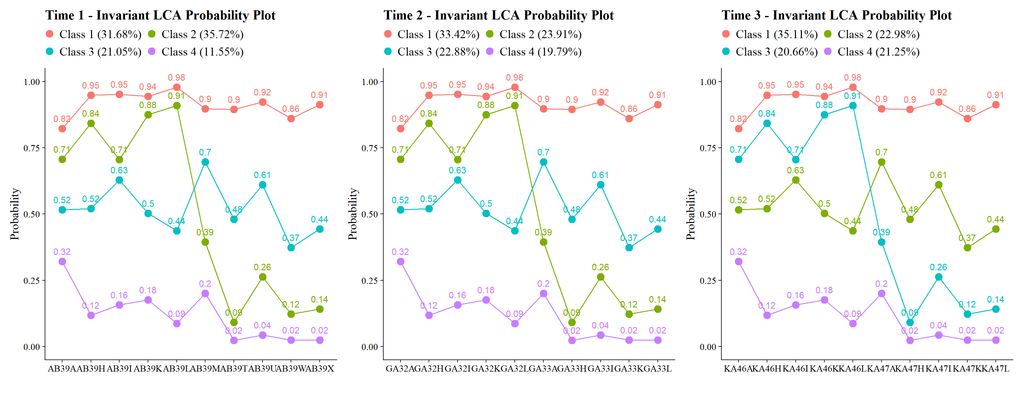
27.12.2 ML STEP 2: Extract Logits and Merge Saved Posterior Data
Extract Classification-Error Logits
inv_step4 <- readModels(here("three_lta", "phase_3","step_1_ml"), quiet = TRUE)

logits_t1 <- as.data.frame(inv_step4$t1_inv_lca.out$class_counts$logitProbs.mostLikely)
logits_t2 <- as.data.frame(inv_step4$t2_inv_lca.out$class_counts$logitProbs.mostLikely)
logits_t3 <- as.data.frame(inv_step4$t3_inv_lca.out$class_counts$logitProbs.mostLikely)
Extract and Merge Saved Posterior Probabilities
savedata_t1 <- as.data.frame(inv_step4$t1_inv_lca.out$savedata) %>%
  rename(cprob11=CPROB1,cprob12=CPROB2,cprob13=CPROB3,cprob14=CPROB4,n1=MLCC1)

savedata_t2 <- as.data.frame(inv_step4$t2_inv_lca.out$savedata) %>%
  rename(cprob21=CPROB1,cprob22=CPROB2,cprob23=CPROB3,cprob24=CPROB4,n2=MLCC2)

savedata_t3 <- as.data.frame(inv_step4$t3_inv_lca.out$savedata) %>%
  rename(cprob31=CPROB1,cprob32=CPROB2,cprob33=CPROB3,cprob34=CPROB4,n3=MLCC3)

savedata_t123 <- savedata_t1 %>%
  full_join(savedata_t2, by = "CASENUM") %>%
  full_join(savedata_t3, by = "CASENUM") %>%
  clean_names() %>% relocate(casenum)

summary(savedata_t123)
#>     casenum         ab39a            ab39h
#>  Min.   :1004   Min.   :0.0000   Min.   :0.0000
#>  1st Qu.:2500   1st Qu.:0.0000   1st Qu.:0.0000
#>  Median :3973   Median :1.0000   Median :1.0000
#>  Mean   :3991   Mean   :0.6881   Mean   :0.7218
#>  3rd Qu.:5505   3rd Qu.:1.0000   3rd Qu.:1.0000
#>  Max.   :6937   Max.   :1.0000   Max.   :1.0000
#>                 NA's   :25       NA's   :56
#>      ab39i           ab39k            ab39l
#>  Min.   :0.000   Min.   :0.0000   Min.   :0.0000
#>  1st Qu.:0.000   1st Qu.:1.0000   1st Qu.:1.0000
#>  Median :1.000   Median :1.0000   Median :1.0000
#>  Mean   :0.653   Mean   :0.7681   Mean   :0.7512
#>  3rd Qu.:1.000   3rd Qu.:1.0000   3rd Qu.:1.0000
#>  Max.   :1.000   Max.   :1.0000   Max.   :1.0000
#>  NA's   :60      NA's   :53       NA's   :50
#>      ab39m            ab39t            ab39u
#>  Min.   :0.0000   Min.   :0.0000   Min.   :0.0000
#>  1st Qu.:0.0000   1st Qu.:0.0000   1st Qu.:0.0000
#>  Median :1.0000   Median :0.0000   Median :0.0000
#>  Mean   :0.6236   Mean   :0.3984   Mean   :0.4924
#>  3rd Qu.:1.0000   3rd Qu.:1.0000   3rd Qu.:1.0000
#>  Max.   :1.0000   Max.   :1.0000   Max.   :1.0000
#>  NA's   :34       NA's   :67       NA's   :57
#>      ab39w            ab39x          minority_x
#>  Min.   :0.0000   Min.   :0.0000   Min.   :0.0000
#>  1st Qu.:0.0000   1st Qu.:0.0000   1st Qu.:0.0000
#>  Median :0.0000   Median :0.0000   Median :0.0000
#>  Mean   :0.3996   Mean   :0.4645   Mean   :0.1704
#>  3rd Qu.:1.0000   3rd Qu.:1.0000   3rd Qu.:0.0000
#>  Max.   :1.0000   Max.   :1.0000   Max.   :1.0000
#>  NA's   :50       NA's   :34       NA's   :105
#>     female_x         mathg7_x       mathg10_x
#>  Min.   :0.0000   Min.   :28.93   Min.   :30.63
#>  1st Qu.:0.0000   1st Qu.:44.84   1st Qu.:58.58
#>  Median :1.0000   Median :53.09   Median :67.71
#>  Mean   :0.5175   Mean   :52.58   Mean   :66.15
#>  3rd Qu.:1.0000   3rd Qu.:59.86   3rd Qu.:75.27
#>  Max.   :1.0000   Max.   :85.07   Max.   :95.26
#>  NA's   :21       NA's   :42      NA's   :532
#>    mathg12_x        cprob11          cprob12
#>  Min.   :27.01   Min.   :0.0000   Min.   :0.0000
#>  1st Qu.:63.40   1st Qu.:0.0000   1st Qu.:0.0030
#>  Median :72.19   Median :0.0080   Median :0.1405
#>  Mean   :71.20   Mean   :0.3169   Mean   :0.3572
#>  3rd Qu.:81.42   3rd Qu.:0.8530   3rd Qu.:0.8210
#>  Max.   :99.30   Max.   :0.9980   Max.   :0.9950
#>  NA's   :1085    NA's   :21       NA's   :21
#>     cprob13          cprob14             n1
#>  Min.   :0.0020   Min.   :0.0000   Min.   :1.000
#>  1st Qu.:0.0090   1st Qu.:0.0000   1st Qu.:1.000
#>  Median :0.0640   Median :0.0000   Median :2.000
#>  Mean   :0.2105   Mean   :0.1155   Mean   :2.093
#>  3rd Qu.:0.2752   3rd Qu.:0.0130   3rd Qu.:3.000
#>  Max.   :0.9990   Max.   :0.9960   Max.   :4.000
#>  NA's   :21       NA's   :21       NA's   :21
#>      ga32a            ga32h            ga32i
#>  Min.   :0.0000   Min.   :0.0000   Min.   :0.0000
#>  1st Qu.:0.0000   1st Qu.:0.0000   1st Qu.:0.0000
#>  Median :1.0000   Median :1.0000   Median :1.0000
#>  Mean   :0.6299   Mean   :0.6493   Mean   :0.6862
#>  3rd Qu.:1.0000   3rd Qu.:1.0000   3rd Qu.:1.0000
#>  Max.   :1.0000   Max.   :1.0000   Max.   :1.0000
#>  NA's   :375      NA's   :387      NA's   :390
#>      ga32k           ga32l            ga33a
#>  Min.   :0.000   Min.   :0.0000   Min.   :0.0000
#>  1st Qu.:0.000   1st Qu.:0.0000   1st Qu.:0.0000
#>  Median :1.000   Median :1.0000   Median :1.0000
#>  Mean   :0.679   Mean   :0.6466   Mean   :0.5917
#>  3rd Qu.:1.000   3rd Qu.:1.0000   3rd Qu.:1.0000
#>  Max.   :1.000   Max.   :1.0000   Max.   :1.0000
#>  NA's   :390     NA's   :382      NA's   :381
#>      ga33h            ga33i            ga33k
#>  Min.   :0.0000   Min.   :0.0000   Min.   :0.0000
#>  1st Qu.:0.0000   1st Qu.:0.0000   1st Qu.:0.0000
#>  Median :0.0000   Median :1.0000   Median :0.0000
#>  Mean   :0.4347   Mean   :0.5251   Mean   :0.4289
#>  3rd Qu.:1.0000   3rd Qu.:1.0000   3rd Qu.:1.0000
#>  Max.   :1.0000   Max.   :1.0000   Max.   :1.0000
#>  NA's   :391      NA's   :391      NA's   :389
#>      ga33l          minority_y        female_y
#>  Min.   :0.0000   Min.   :0.0000   Min.   :0.0000
#>  1st Qu.:0.0000   1st Qu.:0.0000   1st Qu.:0.0000
#>  Median :0.0000   Median :0.0000   Median :1.0000
#>  Mean   :0.4199   Mean   :0.1632   Mean   :0.5254
#>  3rd Qu.:1.0000   3rd Qu.:0.0000   3rd Qu.:1.0000
#>  Max.   :1.0000   Max.   :1.0000   Max.   :1.0000
#>  NA's   :383      NA's   :430      NA's   :373
#>     mathg7_y       mathg10_y       mathg12_y
#>  Min.   :28.93   Min.   :30.63   Min.   :27.01
#>  1st Qu.:46.10   1st Qu.:59.09   1st Qu.:64.00
#>  Median :53.57   Median :67.86   Median :72.56
#>  Mean   :53.20   Mean   :66.41   Mean   :71.63
#>  3rd Qu.:60.09   3rd Qu.:75.30   3rd Qu.:81.73
#>  Max.   :85.07   Max.   :95.26   Max.   :99.30
#>  NA's   :390     NA's   :557     NA's   :1128
#>     cprob21          cprob22          cprob23
#>  Min.   :0.0000   Min.   :0.0000   Min.   :0.0020
#>  1st Qu.:0.0000   1st Qu.:0.0000   1st Qu.:0.0055
#>  Median :0.0035   Median :0.0110   Median :0.0430
#>  Mean   :0.3343   Mean   :0.2391   Mean   :0.2287
#>  3rd Qu.:0.9640   3rd Qu.:0.4000   3rd Qu.:0.3210
#>  Max.   :0.9980   Max.   :0.9920   Max.   :0.9990
#>  NA's   :373      NA's   :373      NA's   :373
#>     cprob24             n2            ka46a
#>  Min.   :0.0000   Min.   :1.000   Min.   :0.000
#>  1st Qu.:0.0000   1st Qu.:1.000   1st Qu.:0.000
#>  Median :0.0000   Median :2.000   Median :1.000
#>  Mean   :0.1979   Mean   :2.275   Mean   :0.567
#>  3rd Qu.:0.1230   3rd Qu.:3.000   3rd Qu.:1.000
#>  Max.   :0.9980   Max.   :4.000   Max.   :1.000
#>  NA's   :373      NA's   :373     NA's   :787
#>      ka46h            ka46i            ka46k
#>  Min.   :0.0000   Min.   :0.0000   Min.   :0.0000
#>  1st Qu.:0.0000   1st Qu.:0.0000   1st Qu.:0.0000
#>  Median :1.0000   Median :1.0000   Median :1.0000
#>  Mean   :0.6733   Mean   :0.7121   Mean   :0.6109
#>  3rd Qu.:1.0000   3rd Qu.:1.0000   3rd Qu.:1.0000
#>  Max.   :1.0000   Max.   :1.0000   Max.   :1.0000
#>  NA's   :796      NA's   :799      NA's   :802
#>      ka46l            ka47a           ka47h
#>  Min.   :0.0000   Min.   :0.000   Min.   :0.000
#>  1st Qu.:0.0000   1st Qu.:0.000   1st Qu.:0.000
#>  Median :1.0000   Median :1.000   Median :0.000
#>  Mean   :0.6513   Mean   :0.552   Mean   :0.485
#>  3rd Qu.:1.0000   3rd Qu.:1.000   3rd Qu.:1.000
#>  Max.   :1.0000   Max.   :1.000   Max.   :1.000
#>  NA's   :803      NA's   :802     NA's   :808
#>      ka47i            ka47k            ka47l
#>  Min.   :0.0000   Min.   :0.0000   Min.   :0.0000
#>  1st Qu.:0.0000   1st Qu.:0.0000   1st Qu.:0.0000
#>  Median :1.0000   Median :0.0000   Median :0.0000
#>  Mean   :0.5645   Mean   :0.3831   Mean   :0.4433
#>  3rd Qu.:1.0000   3rd Qu.:1.0000   3rd Qu.:1.0000
#>  Max.   :1.0000   Max.   :1.0000   Max.   :1.0000
#>  NA's   :807      NA's   :808      NA's   :804
#>     minority          female           mathg7
#>  Min.   :0.0000   Min.   :0.0000   Min.   :28.93
#>  1st Qu.:0.0000   1st Qu.:0.0000   1st Qu.:47.05
#>  Median :0.0000   Median :1.0000   Median :54.23
#>  Mean   :0.1513   Mean   :0.5169   Mean   :54.05
#>  3rd Qu.:0.0000   3rd Qu.:1.0000   3rd Qu.:60.80
#>  Max.   :1.0000   Max.   :1.0000   Max.   :85.07
#>  NA's   :823      NA's   :785      NA's   :793
#>     mathg10         mathg12         cprob31
#>  Min.   :30.63   Min.   :27.01   Min.   :0.0000
#>  1st Qu.:60.66   1st Qu.:63.95   1st Qu.:0.0000
#>  Median :68.83   Median :72.31   Median :0.0060
#>  Mean   :67.49   Mean   :71.59   Mean   :0.3511
#>  3rd Qu.:76.10   3rd Qu.:81.66   3rd Qu.:0.9650
#>  Max.   :95.26   Max.   :99.30   Max.   :0.9980
#>  NA's   :955     NA's   :1137    NA's   :785
#>     cprob32          cprob33          cprob34
#>  Min.   :0.0020   Min.   :0.0000   Min.   :0.0000
#>  1st Qu.:0.0020   1st Qu.:0.0000   1st Qu.:0.0000
#>  Median :0.0400   Median :0.0060   Median :0.0000
#>  Mean   :0.2298   Mean   :0.2066   Mean   :0.2125
#>  3rd Qu.:0.3095   3rd Qu.:0.2480   3rd Qu.:0.2005
#>  Max.   :0.9990   Max.   :0.9910   Max.   :0.9980
#>  NA's   :785      NA's   :785      NA's   :785
#>        n3
#>  Min.   :1.000
#>  1st Qu.:1.000
#>  Median :2.000
#>  Mean   :2.291
#>  3rd Qu.:3.000
#>  Max.   :4.000
#>  NA's   :785
#describe(savedata_t123)
27.12.3 ML STEP 3a: Estimate the Unconditional LTA Model With Fixed Logits
unc_LTA  <- mplusObject(
  TITLE = "Step3a of 3-step",

  VARIABLE =
 "idvariable =casenum;

  nominal=n1 n2 n3;

  usevar = n1 n2 n3;

  classes = c1(4) c2(4) c3(4);

  auxiliary = MINORITY, FEMALE, MATHG7, MATHG10, MATHG12;",

  ANALYSIS =
 "estimator = mlr;
  type = mixture;
  starts = 0;",

  MODEL = glue(
  "%overall%
  c2 on c1;
  c3 on c2;

  Model c1:
    %c1#1%
      [n1#1@{logits_t1[1,1]}];
      [n1#2@{logits_t1[1,2]}];
      [n1#3@{logits_t1[1,3]}];
    %c1#2%
      [n1#1@{logits_t1[2,1]}];
      [n1#2@{logits_t1[2,2]}];
      [n1#3@{logits_t1[2,3]}];
    %c1#3%
      [n1#1@{logits_t1[3,1]}];
      [n1#2@{logits_t1[3,2]}];
      [n1#3@{logits_t1[3,3]}];
    %c1#4%
      [n1#1@{logits_t1[4,1]}];
      [n1#2@{logits_t1[4,2]}];
      [n1#3@{logits_t1[4,3]}];

  Model c2:
    %c2#1%
      [n2#1@{logits_t2[1,1]}];
      [n2#2@{logits_t2[1,2]}];
      [n2#3@{logits_t2[1,3]}];
    %c2#2%
      [n2#1@{logits_t2[2,1]}];
      [n2#2@{logits_t2[2,2]}];
      [n2#3@{logits_t2[2,3]}];
    %c2#3%
      [n2#1@{logits_t2[3,1]}];
      [n2#2@{logits_t2[3,2]}];
      [n2#3@{logits_t2[3,3]}];
    %c2#4%
      [n2#1@{logits_t2[4,1]}];
      [n2#2@{logits_t2[4,2]}];
      [n2#3@{logits_t2[4,3]}];

  Model c3:
    %c3#1%
      [n3#1@{logits_t3[1,1]}];
      [n3#2@{logits_t3[1,2]}];
      [n3#3@{logits_t3[1,3]}];
    %c3#2%
      [n3#1@{logits_t3[2,1]}];
      [n3#2@{logits_t3[2,2]}];
      [n3#3@{logits_t3[2,3]}];
    %c3#3%
      [n3#1@{logits_t3[3,1]}];
      [n3#2@{logits_t3[3,2]}];
      [n3#3@{logits_t3[3,3]}];
    %c3#4%
      [n3#1@{logits_t3[4,1]}];
      [n3#2@{logits_t3[4,2]}];
      [n3#3@{logits_t3[4,3]}];"),

  OUTPUT = "svalues;",

  usevariables = colnames(savedata_t123),
  rdata = savedata_t123)

unc_LTA_fit <- mplusModeler(unc_LTA,
                 dataout=here("three_lta", "phase_3","step_3a_ml", "t123_LTA.dat"),
                 modelout=here("three_lta", "phase_3","step_3a_ml", "unconditional_LTA.inp"),
                 check=TRUE, run = TRUE, hashfilename = FALSE)
27.12.3.1 Plotting Transition Probabilities (Unconditional Model)
source(here("functions","plot_transition.R"))

lta_model <- readModels(here("three_lta", "phase_3","step_3a_ml", "unconditional_LTA.out"))

plot_transition(
  model_name = lta_model,
  facet_labels = c(`1` = "Very Positive", `2` = "Qualified Positive", `3` = "Neutral", `4` = "Less Positive"),
  timepoint_labels = c(`1` = "Grade 7", `2` = "Grade 10", `3` = "Grade 12"),
  class_labels = c(`1` = "Very Positive", `2` = "Qualified Positive", `3` = "Neutral", `4` = "Less Positive")
) +
  labs(title = "Unconditional LTA (ML Three-Step Method)")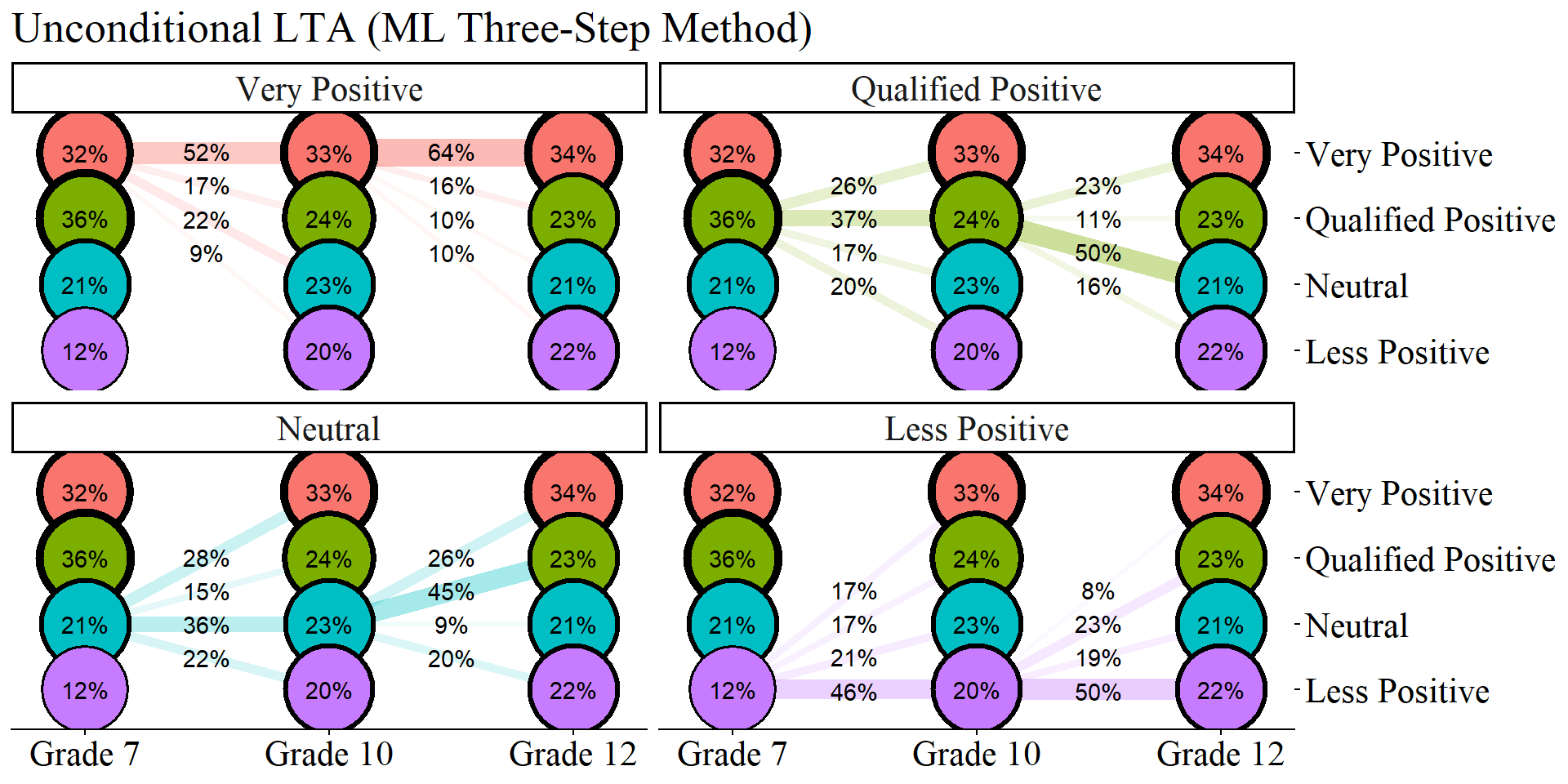
ggsave(here("figures", "unconditional_lta_ml.jpeg"), dpi="retina", height = 6, width = 10, bg = "white", units="in")27.12.4 ML STEP 3b: Estimate the Covariate-Adjusted LTA Model With Fixed Logits
con_LTA  <- mplusObject(
  TITLE = "Step4b of 3-step",

  VARIABLE =
 "idvariable =casenum;

  nominal=n1 n2 n3;

  usevar = n1 n2 n3;

  classes = c1(4) c2(4) c3(4);

  usevar = MINORITY, FEMALE;",

  ANALYSIS =
 "estimator = mlr;
  type = mixture;
  starts = 0;",

  MODEL = glue(
  "%overall%

  c1 ON MINORITY Female;
  c2 ON c1 MINORITY Female;
  c3 ON c2 MINORITY Female;

  Model c1:
    %c1#1%
      [n1#1@{logits_t1[1,1]}];
      [n1#2@{logits_t1[1,2]}];
      [n1#3@{logits_t1[1,3]}];
    %c1#2%
      [n1#1@{logits_t1[2,1]}];
      [n1#2@{logits_t1[2,2]}];
      [n1#3@{logits_t1[2,3]}];
    %c1#3%
      [n1#1@{logits_t1[3,1]}];
      [n1#2@{logits_t1[3,2]}];
      [n1#3@{logits_t1[3,3]}];
    %c1#4%
      [n1#1@{logits_t1[4,1]}];
      [n1#2@{logits_t1[4,2]}];
      [n1#3@{logits_t1[4,3]}];

  Model c2:
    %c2#1%
      [n2#1@{logits_t2[1,1]}];
      [n2#2@{logits_t2[1,2]}];
      [n2#3@{logits_t2[1,3]}];
    %c2#2%
      [n2#1@{logits_t2[2,1]}];
      [n2#2@{logits_t2[2,2]}];
      [n2#3@{logits_t2[2,3]}];
    %c2#3%
      [n2#1@{logits_t2[3,1]}];
      [n2#2@{logits_t2[3,2]}];
      [n2#3@{logits_t2[3,3]}];
    %c2#4%
      [n2#1@{logits_t2[4,1]}];
      [n2#2@{logits_t2[4,2]}];
      [n2#3@{logits_t2[4,3]}];

  Model c3:
    %c3#1%
      [n3#1@{logits_t3[1,1]}];
      [n3#2@{logits_t3[1,2]}];
      [n3#3@{logits_t3[1,3]}];
    %c3#2%
      [n3#1@{logits_t3[2,1]}];
      [n3#2@{logits_t3[2,2]}];
      [n3#3@{logits_t3[2,3]}];
    %c3#3%
      [n3#1@{logits_t3[3,1]}];
      [n3#2@{logits_t3[3,2]}];
      [n3#3@{logits_t3[3,3]}];
    %c3#4%
      [n3#1@{logits_t3[4,1]}];
      [n3#2@{logits_t3[4,2]}];
      [n3#3@{logits_t3[4,3]}];"),

  OUTPUT = "svalues;",

  usevariables = colnames(savedata_t123),
  rdata = savedata_t123)

con_LTA_fit <- mplusModeler(con_LTA,
                 dataout=here("three_lta", "phase_3","step_3b_ml", "t123_LTA.dat"),
                 modelout=here("three_lta", "phase_3","step_3b_ml", "LTA_covariates.inp"),
                 check=TRUE, run = TRUE, hashfilename = FALSE)
27.12.4.1 Covariate Effects Table
lta_cov_model <- readModels(here("three_lta", "phase_3","step_3b_ml", "LTA_covariates.out"))

# REFERENCE CLASS 4
cov <- as.data.frame(lta_cov_model[["parameters"]][["unstandardized"]]) %>%
  filter(param %in% c("MINORITY", "FEMALE")) %>%
  mutate(param = case_when(
            param == "FEMALE" ~ "Gender",
            param == "MINORITY" ~ "URM"),
    se = paste0("(", format(round(se,2), nsmall =2), ")")) %>%
  separate(paramHeader, into = c("Time", "Class"), sep = "#") %>%
  mutate(Class = case_when(
            Class == "1.ON" ~ "Very Positive",
            Class == "2.ON" ~ "Qualified Positive",
            Class == "3.ON" ~ "Neutral"),
         Time = case_when(
            Time == "C1" ~ "7th Grade (T1)",
            Time == "C2" ~ "10th Grade (T2)",
            Time == "C3" ~ "12th Grade (T3)",
         )
         ) %>%
  unite(estimate, est, se, sep = " ") %>%
  select(Time:pval, -est_se) %>%
  mutate(pval = ifelse(pval<0.001, paste0("<.001*"),
                       ifelse(pval<0.05, paste0(scales::number(pval, accuracy = .001), "*"),
                              scales::number(pval, accuracy = .001))))

# Create table

cov_m1 <- cov %>%
  group_by(param, Class) %>%
  gt() %>%
  tab_header(
    title = "Relations Between the Covariates and Latent Class (ML Three-Step Method)") %>%
  tab_footnote(
    footnote = md(
      "Reference Group: Less Positive"
    ),
locations = cells_title()
  ) %>%
  cols_label(
    param = md("Covariate"),
    estimate = md("Estimate (*se*)"),
    pval = md("*p*-value")) %>%
  sub_missing(1:3,
              missing_text = "") %>%
  sub_values(values = c(999.000), replacement = "-") %>%
  cols_align(align = "center") %>%
  opt_align_table_header(align = "left") %>%
  gt::tab_options(table.font.names = "serif")

cov_m1| Relations Between the Covariates and Latent Class (ML Three-Step Method)1 | ||
| Time | Estimate (se) | p-value |
|---|---|---|
| URM - Very Positive | ||
| 7th Grade (T1) | 0.295 (0.40) | 0.459 |
| 10th Grade (T2) | 0.169 (0.33) | 0.611 |
| 12th Grade (T3) | 0.403 (0.37) | 0.273 |
| Gender - Very Positive | ||
| 7th Grade (T1) | -0.398 (0.28) | 0.150 |
| 10th Grade (T2) | -0.124 (0.22) | 0.580 |
| 12th Grade (T3) | 0.155 (0.22) | 0.482 |
| URM - Qualified Positive | ||
| 7th Grade (T1) | -0.174 (0.43) | 0.683 |
| 10th Grade (T2) | 0.429 (0.34) | 0.208 |
| 12th Grade (T3) | 0.818 (0.39) | 0.034* |
| Gender - Qualified Positive | ||
| 7th Grade (T1) | 0.252 (0.29) | 0.380 |
| 10th Grade (T2) | 0.22 (0.25) | 0.379 |
| 12th Grade (T3) | 0.414 (0.26) | 0.105 |
| URM - Neutral | ||
| 7th Grade (T1) | 0.509 (0.47) | 0.279 |
| 10th Grade (T2) | 0.164 (0.39) | 0.673 |
| 12th Grade (T3) | 1.123 (0.40) | 0.005* |
| Gender - Neutral | ||
| 7th Grade (T1) | -0.228 (0.34) | 0.508 |
| 10th Grade (T2) | -0.195 (0.27) | 0.472 |
| 12th Grade (T3) | 0.641 (0.26) | 0.015* |
| 1 Reference Group: Less Positive | ||
27.13 BCH Method
Apply BCH Training Weights for Classification-Error Correction
27.13.1 BCH Step 1: Estimate the Invariant LTA Model and Compute BCH Training Weights
step1_bch  <- mplusObject(
  TITLE = "Step 1 - BCH Method",
  VARIABLE =
     "idvariable=CASENUM;

      usev =
      AB39A AB39H AB39I AB39K AB39L AB39M AB39T AB39U AB39W AB39X
      GA32A GA32H GA32I GA32K GA32L GA33A GA33H GA33I GA33K GA33L
      KA46A KA46H KA46I KA46K KA46L KA47A KA47H KA47I KA47K KA47L;

      categorical =
      AB39A AB39H AB39I AB39K AB39L AB39M AB39T AB39U AB39W AB39X
      GA32A GA32H GA32I GA32K GA32L GA33A GA33H GA33I GA33K GA33L
      KA46A KA46H KA46I KA46K KA46L KA47A KA47H KA47I KA47K KA47L;

      classes = c1(4) c2(4) c3(4);

      auxiliary = MINORITY, FEMALE, MATHG7, MATHG10, MATHG12;",

  ANALYSIS =
   "estimator = mlr;
    type = mixture;
    starts = 0;",

  MODEL =
     "%overall%

  MODEL C1:

     %C1#1%

     [ ab39a$1@-1.53313 ] (1);
     [ ab39h$1@-2.90401 ] (2);
     [ ab39i$1@-2.99575 ] (3);
     [ ab39k$1@-2.83359 ] (4);
     [ ab39l$1@-3.85594 ] (5);
     [ ab39m$1@-2.16372 ] (6);
     [ ab39t$1@-2.13876 ] (7);
     [ ab39u$1@-2.48348 ] (8);
     [ ab39w$1@-1.81515 ] (9);
     [ ab39x$1@-2.35163 ] (10);

     %C1#3%

     [ ab39a$1@-0.06349 ] (11);
     [ ab39h$1@-0.07976 ] (12);
     [ ab39i$1@-0.52495 ] (13);
     [ ab39k$1@-0.01216 ] (14);
     [ ab39l$1@0.25484 ] (15);
     [ ab39m$1@-0.83350 ] (16);
     [ ab39t$1@0.07961 ] (17);
     [ ab39u$1@-0.45274 ] (18);
     [ ab39w$1@0.51840 ] (19);
     [ ab39x$1@0.22569 ] (20);

     %C1#2%

     [ ab39a$1@-0.88292 ] (21);
     [ ab39h$1@-1.67761 ] (22);
     [ ab39i$1@-0.87642 ] (23);
     [ ab39k$1@-1.94409 ] (24);
     [ ab39l$1@-2.31259 ] (25);
     [ ab39m$1@0.42887 ] (26);
     [ ab39t$1@2.29606 ] (27);
     [ ab39u$1@1.02908 ] (28);
     [ ab39w$1@1.97179 ] (29);
     [ ab39x$1@1.80988 ] (30);

     %C1#4%

     [ ab39a$1@0.74744 ] (31);
     [ ab39h$1@2.01287 ] (32);
     [ ab39i$1@1.67957 ] (33);
     [ ab39k$1@1.54221 ] (34);
     [ ab39l$1@2.34965 ] (35);
     [ ab39m$1@1.38217 ] (36);
     [ ab39t$1@3.73153 ] (37);
     [ ab39u$1@3.09927 ] (38);
     [ ab39w$1@3.69495 ] (39);
     [ ab39x$1@3.68803 ] (40);

  MODEL C2:

     %C2#1%

     [ ga32a$1@-1.53313 ] (1);
     [ ga32h$1@-2.90401 ] (2);
     [ ga32i$1@-2.99575 ] (3);
     [ ga32k$1@-2.83359 ] (4);
     [ ga32l$1@-3.85594 ] (5);
     [ ga33a$1@-2.16372 ] (6);
     [ ga33h$1@-2.13876 ] (7);
     [ ga33i$1@-2.48348 ] (8);
     [ ga33k$1@-1.81515 ] (9);
     [ ga33l$1@-2.35163 ] (10);

     %C2#3%

     [ ga32a$1@-0.06349 ] (11);
     [ ga32h$1@-0.07976 ] (12);
     [ ga32i$1@-0.52495 ] (13);
     [ ga32k$1@-0.01216 ] (14);
     [ ga32l$1@0.25484 ] (15);
     [ ga33a$1@-0.83350 ] (16);
     [ ga33h$1@0.07961 ] (17);
     [ ga33i$1@-0.45274 ] (18);
     [ ga33k$1@0.51840 ] (19);
     [ ga33l$1@0.22569 ] (20);

     %C2#2%

     [ ga32a$1@-0.88292 ] (21);
     [ ga32h$1@-1.67761 ] (22);
     [ ga32i$1@-0.87642 ] (23);
     [ ga32k$1@-1.94409 ] (24);
     [ ga32l$1@-2.31259 ] (25);
     [ ga33a$1@0.42887 ] (26);
     [ ga33h$1@2.29606 ] (27);
     [ ga33i$1@1.02908 ] (28);
     [ ga33k$1@1.97179 ] (29);
     [ ga33l$1@1.80988 ] (30);

     %C2#4%

     [ ga32a$1@0.74744 ] (31);
     [ ga32h$1@2.01287 ] (32);
     [ ga32i$1@1.67957 ] (33);
     [ ga32k$1@1.54221 ] (34);
     [ ga32l$1@2.34965 ] (35);
     [ ga33a$1@1.38217 ] (36);
     [ ga33h$1@3.73153 ] (37);
     [ ga33i$1@3.09927 ] (38);
     [ ga33k$1@3.69495 ] (39);
     [ ga33l$1@3.68803 ] (40);

  MODEL C3:

     %C3#1%

     [ ka46a$1@-1.53313 ] (1);
     [ ka46h$1@-2.90401 ] (2);
     [ ka46i$1@-2.99575 ] (3);
     [ ka46k$1@-2.83359 ] (4);
     [ ka46l$1@-3.85594 ] (5);
     [ ka47a$1@-2.16372 ] (6);
     [ ka47h$1@-2.13876 ] (7);
     [ ka47i$1@-2.48348 ] (8);
     [ ka47k$1@-1.81515 ] (9);
     [ ka47l$1@-2.35163 ] (10);

     %C3#3%

     [ ka46a$1@-0.06349 ] (11);
     [ ka46h$1@-0.07976 ] (12);
     [ ka46i$1@-0.52495 ] (13);
     [ ka46k$1@-0.01216 ] (14);
     [ ka46l$1@0.25484 ] (15);
     [ ka47a$1@-0.83350 ] (16);
     [ ka47h$1@0.07961 ] (17);
     [ ka47i$1@-0.45274 ] (18);
     [ ka47k$1@0.51840 ] (19);
     [ ka47l$1@0.22569 ] (20);

     %C3#2%

     [ ka46a$1@-0.88292 ] (21);
     [ ka46h$1@-1.67761 ] (22);
     [ ka46i$1@-0.87642 ] (23);
     [ ka46k$1@-1.94409 ] (24);
     [ ka46l$1@-2.31259 ] (25);
     [ ka47a$1@0.42887 ] (26);
     [ ka47h$1@2.29606 ] (27);
     [ ka47i$1@1.02908 ] (28);
     [ ka47k$1@1.97179 ] (29);
     [ ka47l$1@1.80988 ] (30);

     %C3#4%

     [ ka46a$1@0.74744 ] (31);
     [ ka46h$1@2.01287 ] (32);
     [ ka46i$1@1.67957 ] (33);
     [ ka46k$1@1.54221 ] (34);
     [ ka46l$1@2.34965 ] (35);
     [ ka47a$1@1.38217 ] (36);
     [ ka47h$1@3.73153 ] (37);
     [ ka47i$1@3.09927 ] (38);
     [ ka47k$1@3.69495 ] (39);
     [ ka47l$1@3.68803 ] (40);",

  SAVEDATA =
   "File=bch_savedata.dat;
    Save=bchweights;",

  OUTPUT = "sampstat svalues",

  usevariables = colnames(lsay_data),
  rdata = lsay_data)

step1_fit_bch <- mplusModeler(step1_bch,
                            dataout=here("three_lta", "phase_3", "step_1_bch", "step1.dat"),
                            modelout=here("three_lta", "phase_3", "step_1_bch", "step1_bch.inp") ,
                            check=TRUE, run = TRUE, hashfilename = FALSE)
27.13.1.1 Diagnostic Plot of the Invariant BCH Model
source(here("functions","plot_lta.R"))

inv_bch <- readModels(here("three_lta", "phase_3","step_1_bch"), quiet = TRUE)

plot_lta(inv_bch)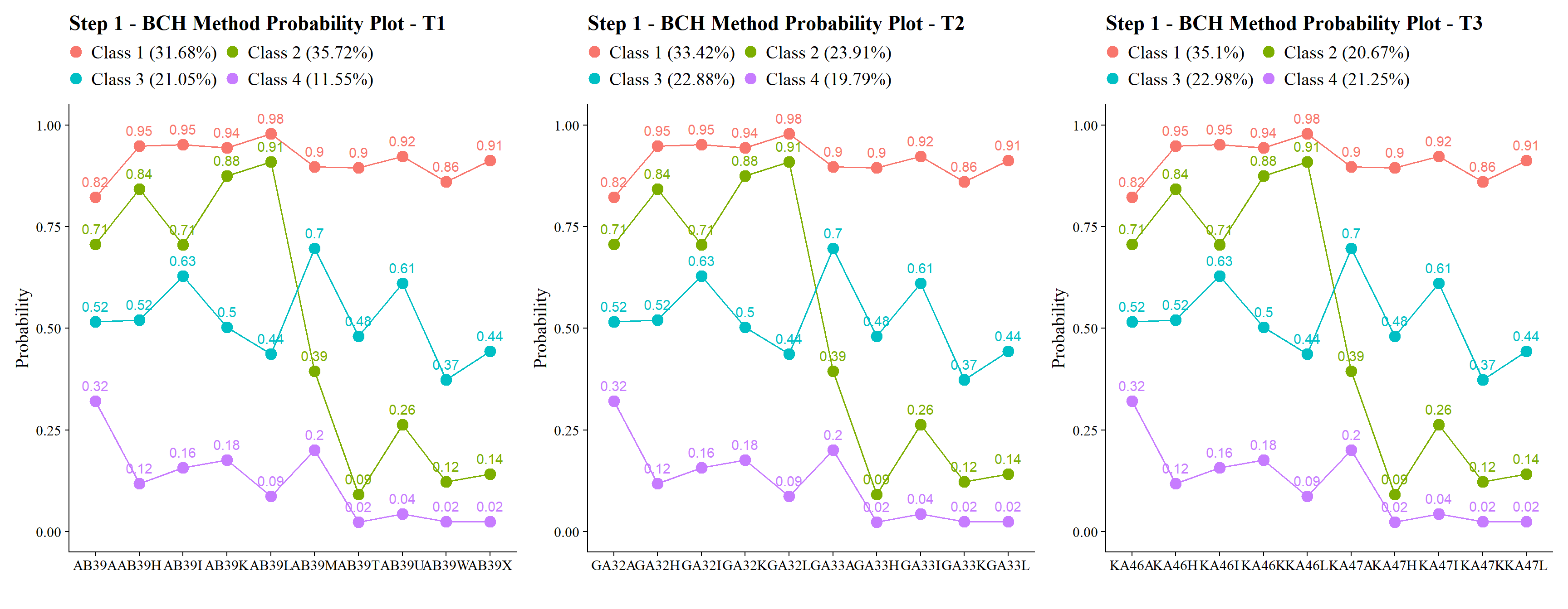
27.13.2 BCH Step 2: Extract BCH weights
bch_savedata <- as.data.frame(inv_bch$savedata)
#summary(bch_savedata)
27.13.3 BCH Step 3a: Estimate the Unconditional LTA Model Using BCH Weights
step3_bch  <- mplusObject(
  TITLE = "Step 3 - BCH Method",

  VARIABLE =
 "usevar = BCHW1-BCHW64;

  training = BCHW1-BCHW64(bch);

  classes = c1(4) c2(4) c3(4);" ,

  ANALYSIS =
 "type = mixture;
  starts = 0;",

  MODEL = glue(
  "%overall%

  c2 ON c1;
  c3 ON c2;"),

  usevariables = colnames(bch_savedata),
  rdata = bch_savedata)

step3_fit_bch <- mplusModeler(step3_bch,
               dataout=here("three_lta", "phase_3", "step_3a_bch", "step3.dat"),
               modelout=here("three_lta", "phase_3", "step_3a_bch", "unconditional_bch.inp"),
               check=TRUE, run = TRUE, hashfilename = FALSE)
27.13.3.1 Plotting BCH Transition Probabilities
source(here("functions","plot_transition.R"))

lta_model <- readModels(here("three_lta", "phase_3", "step_3a_bch", "unconditional_bch.out"))

plot_transition(
  model_name = lta_model,
  facet_labels = c(`1` = "Very Positive", `2` = "Qualified Positive", `3` = "Neutral", `4` = "Less Positive"),
  timepoint_labels = c(`1` = "Grade 7", `2` = "Grade 10", `3` = "Grade 12"),
  class_labels = c(`1` = "Very Positive", `2` = "Qualified Positive", `3` = "Neutral", `4` = "Less Positive")
) +
  labs(title = "Unconditional LTA (BCH Method)")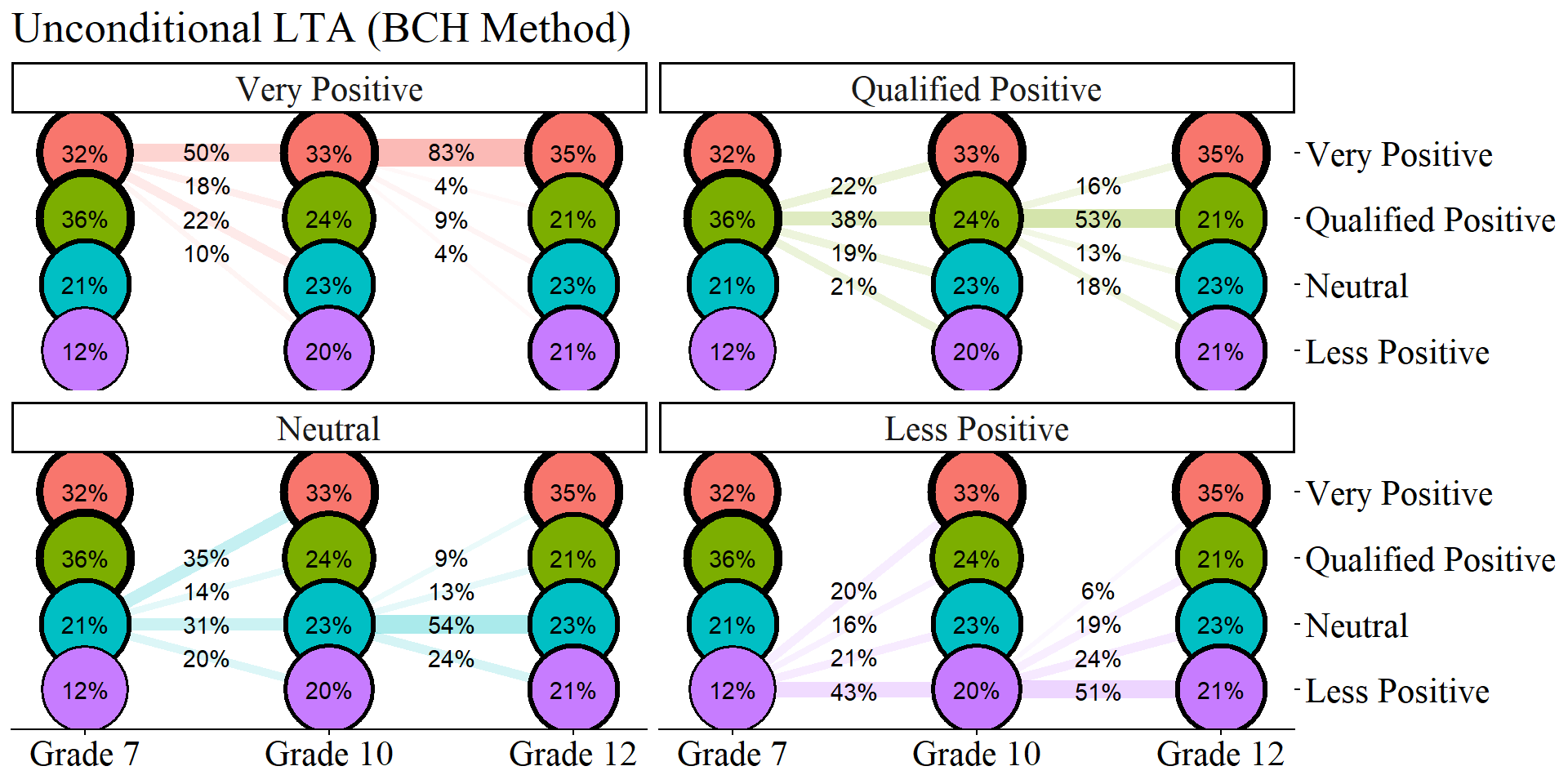
ggsave(here("figures", "unconditional_lta_bch.jpeg"), dpi="retina", height = 6, width = 10, bg = "white", units="in")27.13.4 BCH Step 3b: Estimate the Covariate-Adjusted LTA Model Using BCH Weights
step3_bch  <- mplusObject(
  TITLE = "Step 3 - BCH Method",

  VARIABLE =
 "usevar = BCHW1-BCHW64 MINORITY, FEMALE;

  training = BCHW1-BCHW64(bch);

  classes = c1(4) c2(4) c3(4);" ,

  ANALYSIS =
 "estimator = mlr;
  type = mixture;
  starts = 0;",

  MODEL =
  glue(
 " %OVERALL%

  c1 ON MINORITY Female;
  c2 ON c1 MINORITY Female;
  c3 ON c2 MINORITY Female;"),

  usevariables = colnames(bch_savedata),
  rdata = bch_savedata)

step3_fit_bch <- mplusModeler(step3_bch,
               dataout=here("three_lta", "phase_3", "step_3b_bch", "step3.dat"),
               modelout=here("three_lta", "phase_3", "step_3b_bch", "bch_covariates.inp"),
               check=TRUE, run = TRUE, hashfilename = FALSE)
27.13.4.1 Covariate Table: BCH Method
lta_cov_model <- readModels(here("three_lta", "phase_3", "step_3b_bch", "bch_covariates.out"))

# REFERENCE CLASS 4
cov <- as.data.frame(lta_cov_model[["parameters"]][["unstandardized"]]) %>%
  filter(param %in% c("MINORITY", "FEMALE")) %>%
  mutate(param = case_when(
            param == "FEMALE" ~ "Gender",
            param == "MINORITY" ~ "URM"),
    se = paste0("(", format(round(se,2), nsmall =2), ")")) %>%
  separate(paramHeader, into = c("Time", "Class"), sep = "#") %>%
  mutate(Class = case_when(
            Class == "1.ON" ~ "Very Positive",
            Class == "2.ON" ~ "Qualified Positive",
            Class == "3.ON" ~ "Neutral"),
         Time = case_when(
            Time == "C1" ~ "7th Grade (T1)",
            Time == "C2" ~ "10th Grade (T2)",
            Time == "C3" ~ "12th Grade (T3)",
         )
         ) %>%
  unite(estimate, est, se, sep = " ") %>%
  select(Time:pval, -est_se) %>%
  mutate(pval = ifelse(pval<0.001, paste0("<.001*"),
                       ifelse(pval<0.05, paste0(scales::number(pval, accuracy = .001), "*"),
                              scales::number(pval, accuracy = .001))))


# Create table

cov_m1 <- cov %>%
  group_by(param, Class) %>%
  gt() %>%
  tab_header(
    title = "Relations Between the Covariates and Latent Class (BCH Method)") %>%
  tab_footnote(
    footnote = md(
      "Reference Group: Less Positive"
    ),
locations = cells_title()
  ) %>%
  cols_label(
    param = md("Covariate"),
    estimate = md("Estimate (*se*)"),
    pval = md("*p*-value")) %>%
  sub_missing(1:3,
              missing_text = "") %>%
  sub_values(values = c(999.000), replacement = "-") %>%
  cols_align(align = "center") %>%
  opt_align_table_header(align = "left") %>%
  gt::tab_options(table.font.names = "serif")

cov_m1| Relations Between the Covariates and Latent Class (BCH Method)1 | ||
| Time | Estimate (se) | p-value |
|---|---|---|
| URM - Very Positive | ||
| 7th Grade (T1) | 0.225 (0.27) | 0.406 |
| 10th Grade (T2) | 0.442 (0.27) | 0.100 |
| 12th Grade (T3) | 0.809 (0.60) | 0.175 |
| Gender - Very Positive | ||
| 7th Grade (T1) | -0.655 (0.19) | 0.001* |
| 10th Grade (T2) | -0.091 (0.20) | 0.641 |
| 12th Grade (T3) | 0.338 (0.45) | 0.457 |
| URM - Qualified Positive | ||
| 7th Grade (T1) | 0.096 (0.28) | 0.736 |
| 10th Grade (T2) | 0.444 (0.27) | 0.105 |
| 12th Grade (T3) | 1.099 (0.40) | 0.006* |
| Gender - Qualified Positive | ||
| 7th Grade (T1) | 0.1 (0.20) | 0.621 |
| 10th Grade (T2) | 0.411 (0.20) | 0.039* |
| 12th Grade (T3) | 0.623 (0.27) | 0.022* |
| URM - Neutral | ||
| 7th Grade (T1) | 0.515 (0.32) | 0.103 |
| 10th Grade (T2) | 0.145 (0.31) | 0.640 |
| 12th Grade (T3) | 0.822 (0.40) | 0.039* |
| Gender - Neutral | ||
| 7th Grade (T1) | -0.431 (0.24) | 0.069 |
| 10th Grade (T2) | 0.062 (0.21) | 0.771 |
| 12th Grade (T3) | 0.372 (0.26) | 0.152 |
| 1 Reference Group: Less Positive | ||